AutoML
By now every model you train comes with knobs. Model Selection explained what the knobs do (bias against variance) and put several model families into one GridSearchCV; Cross-Validation showed how to compare the results honestly, and why the winner of a search always looks better than it is. What neither lesson asked is how to spend the search budget. A grid tries every combination of a few values; with five hyperparameters and five values each, that is 3,125 cross-validations, most of them in regions that were obviously bad after the first dozen.
Hyperparameter optimization treats the search itself as an optimization problem, and AutoML pushes the same idea to the whole pipeline: preprocessing, model family, hyperparameters and the final ensemble. This lesson builds the methods from the inside, each one measured: random search against a grid (Bergstra & Bengio's argument, simulated), Bayesian optimization with a Gaussian process and expected improvement computed by hand, TPE and Optuna, successive halving and Hyperband. Then it measures the two ways an automated search fails: it optimizes a leak as eagerly as a signal, and the longer it searches, the more its own score flatters it.
Every number below comes from the code blocks or from the figure scripts next to this page.
The lesson tells this in five stages, drawn below: 1. frame the search, an expensive, noisy black box and the space it is searched over; 2. grid or random, the two searches that remember nothing; 3. a search that learns, Bayesian optimization and TPE, which use the past trials to choose the next one; 4. stop bad trials early, pruning, successive halving and Hyperband; 5. automate, then check, the whole pipeline and what no search can fix. Each stage links to its section, and in the slides a strip at the bottom shows which stage you are in.
- Frame the searchan expensive, noisy black box; the search space
- Grid or randomBergstra & Bengio, measured
- A search that learnsBayesian optimization, TPE, Optuna
- Stop bad trials earlypruning, successive halving, Hyperband
- Automate, then checkthe whole pipeline, leaks, a flattering score
Slides
Click the slides and use the ← → arrows to navigate; F goes full screen and Esc shows every slide. Open the slides in a new tab
Tuning is an optimization problem
An expensive, noisy black box
Stage 1. Call \(\lambda\) a configuration (a learning rate, a tree size, a leaf size...) and \(f(\lambda)\) its cross-validated score. Tuning means finding the \(\lambda\) with the largest \(f(\lambda)\). Written like that, it looks like the problems of gradient descent, but three things make it different. Here is one call to \(f\) on kc1, a NASA data set of 2,109 software modules described by 21 code metrics (lines of code, cyclomatic complexity, operator counts...), where the target says whether a defect was later found in the module:
import numpy as np
from sklearn.datasets import fetch_openml
from sklearn.ensemble import HistGradientBoostingClassifier
from sklearn.model_selection import StratifiedKFold, cross_val_score, train_test_split

kc1 = fetch_openml(data_id=1067, as_frame=True)            # 2,109 modules of a NASA flight system
X, y = kc1.data, (kc1.target == 'true').astype(int)         # 1 = a defect was later found in it
X_dev, X_test, y_dev, y_test = train_test_split(X, y, test_size=0.2, stratify=y, random_state=0)
print(X_dev.shape, f"defective: {y_dev.mean():.1%}")


def evaluate(params, seed=0):
    """One call to the black box: the 5-fold CV ROC AUC of a boosted model with these settings."""
    cv = StratifiedKFold(n_splits=5, shuffle=True, random_state=seed)
    model = HistGradientBoostingClassifier(random_state=0, **params)
    return cross_val_score(model, X_dev, y_dev, cv=cv, scoring='roc_auc').mean()


for name, params in [('defaults', {}),
                     ('small, slow trees', {'learning_rate': 0.03, 'max_leaf_nodes': 8,
                                            'min_samples_leaf': 50})]:
    runs = [evaluate(params, seed) for seed in range(5)]    # same settings, 5 fold shuffles
    print(f"{name:17s} {np.round(runs, 3)}  mean {np.mean(runs):.3f}")
(1687, 21) defective: 15.5%
defaults          [0.76  0.776 0.767 0.769 0.769]  mean 0.768
small, slow trees [0.795 0.806 0.804 0.803 0.805]  mean 0.803
- Expensive. Each call is 5 model fits. Here they take a fraction of a second; on a real project, one call can take minutes or hours, so the number of calls, not the arithmetic around them, is the budget.
- Noisy. The same configuration, cross-validated with 5 different shuffles of the folds, scores anywhere from 0.760 to 0.776. The difference between the two configurations (0.768 against 0.803) is real, but a difference of 0.01 between two others might not be.
- A black box. There is no gradient of the CV score with respect to
min_samples_leaf: the function can only be evaluated. Several knobs are integers or categories, and some only exist when another knob takes a certain value.
A tuning method is a rule for choosing the next \(\lambda\) to evaluate, given the ones already evaluated. The methods below differ only in that rule.
Designing the search space
Before any method runs, someone has to say which values are allowed. Two decisions matter more than the choice of method.
Scale. A learning rate of 0.001 and one of 0.01 are as different as 0.1 and 1: what matters is the ratio. Sampling uniformly between 0.001 and 1 ignores this:
from scipy.stats import loguniform, uniform

u = uniform(0.001, 1 - 0.001).rvs(100_000, random_state=0)   # uniform on [0.001, 1]
lu = loguniform(0.001, 1).rvs(100_000, random_state=0)       # uniform on the log scale
for lo, hi in [(0.001, 0.01), (0.01, 0.1), (0.1, 1)]:
    print(f"learning rate in [{lo}, {hi}):  uniform {np.mean((u >= lo) & (u < hi)):5.1%}"
          f"   log-uniform {np.mean((lu >= lo) & (lu < hi)):5.1%}")
learning rate in [0.001, 0.01):  uniform  0.9%   log-uniform 33.5%
learning rate in [0.01, 0.1):  uniform  9.1%   log-uniform 33.2%
learning rate in [0.1, 1):  uniform 90.0%   log-uniform 33.3%
By hand: the interval \([0.001, 0.01)\) is \(0.009 / 0.999 = 0.9\%\) of the uniform range, while on the log scale each decade is one third of \(\log_{10}(1/0.001) = 3\) decades. A uniform search spends 90% of its budget on learning rates above 0.1 and almost nothing on the decade where, on kc1, the best boosted models live (see the halving figure below: the best configurations have learning rates between 0.01 and 0.03). Rule: anything that acts multiplicatively (learning rates, regularization strengths C and alpha, the number of leaves or of neighbors) gets a log scale: loguniform in scikit-learn, log=True in Optuna.
Conditional parameters. Some hyperparameters only exist in some configurations: C belongs to the logistic regression, max_leaf_nodes to the booster, gamma to an RBF kernel. A single grid over all of them would pair every C with every tree size, fitting the same logistic regression again and again. Model Selection solved it with a list of grids, one per family. The search space is really a tree: first choose the family, then that family's knobs. The Optuna code below writes that tree as an if.
Grid or random? Bergstra & Bengio, measured
Stage 2. Model Selection closed with a claim from Bergstra & Bengio (2012): when only a few hyperparameters really matter, random combinations cover those few much better than a grid. Here is the argument, measured. Take a score that depends on one hyperparameter, \(x_1\), through a bump of width 0.05 around an unknown best value \(c\); the other \(d - 1\) hyperparameters do nothing. Both methods get the same budget \(B\). A grid with \(k\) values per axis costs \(B = k^d\) evaluations, but it tries the important parameter at only \(k\) distinct values. Random search tries it at \(B\) distinct values, whatever \(d\) is.
By hand: with \(k\) grid values at \(\tfrac{1}{2k}, \tfrac{3}{2k}, \dots\), the optimum is at most \(\tfrac{1}{2k}\) away from the nearest one, and on average \(\tfrac{1}{4k}\): 0.083 for \(k = 3\). With \(B\) random values, the nearest one is on average about \(\tfrac{1}{2(B + 1)}\) away: 0.05 for \(B = 9\), 0.006 for \(B = 81\). Averaged over 4,000 problems with \(c\) drawn at random:
rng = np.random.default_rng(0)
c = rng.uniform(0, 1, 4000)         # 4,000 problems: the best value of x1 can be anywhere
W = 0.05                            # the score is a bump of width 0.05 around it


def distance_and_score(x1):
    """Mean distance from the optimum to the nearest x1 tried, and mean best score found."""
    dist = np.abs(x1 - c[:, None]).min(axis=1)
    return dist.mean(), np.exp(-dist ** 2 / (2 * W ** 2)).mean()


print(" d  budget  x1 values in grid   distance: grid  random   best score: grid  random")
for d, k in [(2, 3), (2, 9), (3, 3), (4, 3), (4, 4)]:
    B = k ** d                                          # a k × k × ... grid
    grid_x1 = (np.arange(k) + 0.5) / k                  # the k values the grid gives x1
    rand_x1 = rng.uniform(0, 1, (len(c), B))            # B random values of x1, fresh per problem
    (dg, sg), (dr, sr) = distance_and_score(grid_x1), distance_and_score(rand_x1)
    print(f"{d:2d}  {B:6d}  {k:17d}   {dg:14.3f}  {dr:6.3f}   {sg:16.3f}  {sr:6.3f}")
 d  budget  x1 values in grid   distance: grid  random   best score: grid  random
 2       9                  3            0.083   0.054              0.378   0.629
 2      81                  9            0.028   0.006              0.824   0.985
 3      27                  3            0.083   0.018              0.378   0.900
 4      81                  3            0.083   0.006              0.378   0.986
 4     256                  4            0.062   0.002              0.501   0.998
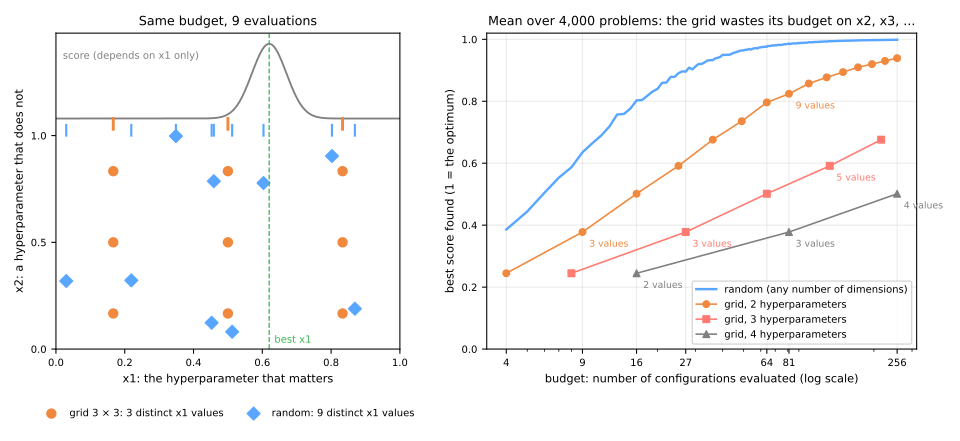
With 9 evaluations in two dimensions, the grid lands on average 0.083 from the optimum and scores 0.378; random search lands 0.054 away and scores 0.629. The gap explodes with the number of useless dimensions. With 81 evaluations over four hyperparameters, the grid still tries \(x_1\) at only 3 values, so it scores exactly what the 3 × 3 grid scored (0.378), while random search is at 0.986. The grid pays for every irrelevant axis with a multiplication of its cost; random search pays nothing, because an irrelevant axis does not change where its points fall on the relevant one.
Real searches are like this. Bergstra & Bengio fitted a model of the validation score to their neural-network experiments and found that, on each data set, only a few of the hyperparameters really mattered, and that which ones mattered changed from one data set to the next, so you cannot design the grid around them in advance. A grid is still fine for one or two hyperparameters you understand (a C curve, a k curve). Beyond that, random search is the honest baseline that every cleverer method must beat.
See it on one problem at a time. Start at a budget of 9, count the distinct values of \(x_1\) each method tries, then raise the budget and press new problem a few times; the line at the bottom right redoes the average over 2,000 problems:
On a single problem the grid sometimes wins, when one of its few columns happens to fall on the bump; on average it never does, because a \(k \times k\) grid pays \(k^2\) evaluations for \(k\) values of the only hyperparameter that matters. The simulator's second mode, successive halving, previews the tournament of a later section: its scores are synthetic, but it reproduces the trap described there, where a budget counted in trees eliminates the slow learners first.
Bayesian optimization: a search that learns
Stage 3. Random search ignores everything it has already seen: the 27th configuration is drawn exactly like the first. When each evaluation costs an hour, that is wasteful. Bayesian optimization (Jones, Schonlau & Welch, 1998; Snoek, Larochelle & Adams, 2012, for machine learning) uses the evaluations so far to decide where to look next, in a loop:
- fit a cheap surrogate model to the pairs (configuration, score) seen so far. The surrogate predicts the score anywhere, with an uncertainty;
- choose the next configuration by maximizing an acquisition function, which trades off exploitation (where the surrogate predicts a high score) against exploration (where it is unsure);
- evaluate that configuration, add it to the history, repeat.
To watch it work, we need a black box whose truth we know. The function below stands in for a validation score as a function of one (log-scaled) hyperparameter \(x\): a broad peak of 0.78 at 0.25 and a higher, narrower one of 0.82 at 0.72.
The surrogate
The usual surrogate is a Gaussian process (GP). You do not need its mathematics to use it: a GP predicts, at every \(x\), a mean \(\mu(x)\) and a standard deviation \(\sigma(x)\). The mean passes through the evaluated points; the standard deviation is zero there and grows with the distance from them. How fast it grows is set by the kernel's length scale: with 0.15, the surrogate assumes that points closer than about 0.15 have similar scores.
from scipy.stats import norm
from sklearn.gaussian_process import GaussianProcessRegressor
from sklearn.gaussian_process.kernels import RBF


def score(x):
    """A stand-in for an expensive validation score, as a function of one hyperparameter."""
    return 0.70 + 0.08 * np.exp(-((x - 0.25) / 0.10) ** 2) + 0.12 * np.exp(-((x - 0.72) / 0.06) ** 2)


X_seen = np.array([0.15, 0.35, 0.95])                       # three evaluations so far
y_seen = score(X_seen)
gp = GaussianProcessRegressor(kernel=RBF(length_scale=0.15), normalize_y=True, optimizer=None)
gp.fit(X_seen.reshape(-1, 1), y_seen)
print('evaluated:', X_seen, '->', y_seen.round(5))
for x in [0.25, 0.55, 0.72]:
    mu, sd = gp.predict([[x]], return_std=True)
    print(f"x = {x}: surrogate mean {mu[0]:.5f}, sd {sd[0]:.5f}")
evaluated: [0.15 0.35 0.95] -> [0.72943 0.72943 0.7    ]
x = 0.25: surrogate mean 0.73076, sd 0.00419
x = 0.55: surrogate mean 0.72212, sd 0.01246
x = 0.72: surrogate mean 0.71390, sd 0.01318
Three points look very different to the surrogate. At 0.25, between two evaluated points, it is nearly sure: mean 0.73076, just above the best score so far, \(f^+ = 0.72943\), with a tiny standard deviation. At 0.55 and 0.72, far from any evaluation, the means are below \(f^+\) but the uncertainty is three times larger. (The surrogate knows nothing of the peak at 0.72: nothing has been evaluated near it.)
The acquisition function: expected improvement, by hand
Which of the three deserves the next evaluation? Expected improvement (EI) asks: if the score at \(x\) is a normal variable with mean \(\mu\) and standard deviation \(\sigma\), how much will it beat \(f^+\) on average, counting a failure to beat it as zero? The answer has a closed form, with \(z = (\mu - f^+)/\sigma\), \(\Phi\) the normal cumulative distribution and \(\varphi\) its density:
The first term rewards a high mean (exploitation), the second a large uncertainty (exploration). With the numbers printed above (\(\Phi\) and \(\varphi\) from a normal table):
| \(x\) | \(\mu - f^+\) | \(\sigma\) | \(z\) | \(\Phi(z)\) | \(\varphi(z)\) | \((\mu - f^+)\Phi(z)\) | \(\sigma\varphi(z)\) | EI |
|---|---|---|---|---|---|---|---|---|
| 0.25 | +0.00133 | 0.00419 | +0.32 | 0.626 | 0.379 | +0.00083 | 0.00159 | 0.00242 |
| 0.55 | −0.00731 | 0.01246 | −0.59 | 0.278 | 0.335 | −0.00203 | 0.00417 | 0.00214 |
| 0.72 | −0.01553 | 0.01318 | −1.18 | 0.119 | 0.199 | −0.00185 | 0.00262 | 0.00077 |
At 0.25 the mean does the work; at 0.55 the uncertainty does, and it almost wins. The library agrees:
def expected_improvement(x, gp, best):
    mu, sd = gp.predict(np.reshape(x, (-1, 1)), return_std=True)
    z = (mu - best) / sd
    return (mu - best) * norm.cdf(z) + sd * norm.pdf(z)


xs = np.linspace(0, 1, 201)                                 # the candidates we can afford to score
ei = expected_improvement(xs, gp, y_seen.max())
for x in [0.25, 0.55, 0.72]:
    print(f"EI({x}) = {expected_improvement(x, gp, y_seen.max())[0]:.4f}")
print(f"largest EI at x = {xs[ei.argmax()]:.3f}")
Computing EI on 201 candidates costs nothing next to one cross-validation: that is the whole trade. The expensive function is evaluated once per iteration; the cheap surrogate is queried thousands of times.
Four iterations
def bayes_opt(X_seen, n_iter, length_scale=0.15):
    """Fit the surrogate, evaluate the argmax of EI, repeat."""
    y_seen = score(X_seen)
    for _ in range(n_iter):
        gp = GaussianProcessRegressor(kernel=RBF(length_scale), normalize_y=True, optimizer=None)
        gp.fit(X_seen.reshape(-1, 1), y_seen)
        x_next = xs[np.argmax(expected_improvement(xs, gp, y_seen.max()))]
        X_seen, y_seen = np.append(X_seen, x_next), np.append(y_seen, score(x_next))
    return X_seen, y_seen


X_bo, y_bo = bayes_opt(np.array([0.15, 0.35, 0.95]), n_iter=4)
print('x tried:', X_bo[3:], '-> score', y_bo[3:].round(3))
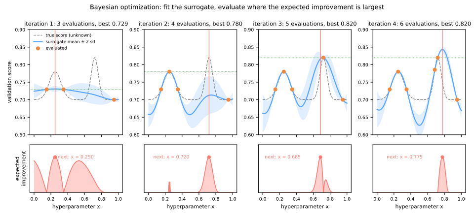
Each column is one iteration: the surrogate (blue band: mean ± 2 standard deviations) with the true score in dashed gray, and underneath, the expected improvement with its maximum marked. Iteration 1 exploits: it evaluates 0.25 and finds 0.780. Now the left peak is known, so its EI collapses, and the largest EI sits in the wide, unexplored gap between 0.4 and 0.9. Iteration 2 explores there, evaluates 0.72 and finds the optimum, 0.820. Iterations 3 and 4 check its neighbors, 0.685 and 0.775. After five evaluations in all, the search has found the best configuration; random search would need, on average, about 28 draws to fall within \(\pm 0.018\) of 0.72, the band where the score exceeds 0.81.
The surrogate's assumptions matter
That run was a good one. Repeat it from 100 random starting triples, and compare with random search, all with 30 evaluations:
rng = np.random.default_rng(0)
first_hit = {'BO, length scale 0.15': [], 'BO, length scale 0.10': [], 'random search': []}
for run in range(100):
    start = rng.uniform(0, 1, 3)                                  # 3 random evaluations to begin
    runs = {'BO, length scale 0.15': bayes_opt(start, 27, 0.15)[1],
            'BO, length scale 0.10': bayes_opt(start, 27, 0.10)[1],
            'random search': score(rng.uniform(0, 1, 30))}
    for name, ys in runs.items():                                 # 30 evaluations each
        hits = np.flatnonzero(ys >= 0.81)                         # within 0.01 of the optimum
        first_hit[name].append(hits[0] + 1 if len(hits) else np.inf)
for name, n in first_hit.items():
    n = np.array(n)
    print(f"{name:22s} reached 0.81 within 10 / 20 / 30 evaluations: "
          f"{np.mean(n <= 10):.0%} / {np.mean(n <= 20):.0%} / {np.mean(n <= 30):.0%}")
BO, length scale 0.15  reached 0.81 within 10 / 20 / 30 evaluations: 40% / 65% / 65%
BO, length scale 0.10  reached 0.81 within 10 / 20 / 30 evaluations: 61% / 92% / 92%
random search          reached 0.81 within 10 / 20 / 30 evaluations: 37% / 54% / 65%
With a length scale of 0.15, Bayesian optimization is ahead of random search at 10 evaluations (40% of runs against 37%)... and then stops improving: 35% of its runs have still not found the high peak after 30 evaluations. The surrogate is too sure that the score is smooth. Once the broad peak at 0.25 is well explored and a few points on the right came back at 0.70, it predicts a flat, certain 0.70 over the narrow peak (width 0.06) and puts no expected improvement there. With a length scale of 0.10, closer to the real width of the peak, 92% of the runs find it within 20 evaluations, against 54% for random search.
So the surrogate is a model like any other, and a wrong model makes wrong decisions confidently. Real implementations do not fix the length scale by hand as we did: they fit the kernel's parameters to the evaluations by maximum likelihood at every iteration, and many add a little forced exploration. They also have to deal with what a GP handles badly: integer and categorical hyperparameters, conditional ones, and more than a dozen dimensions. That is what the next method was designed for.
TPE and Optuna
TPE: a density for the good trials, one for the rest
The Tree-structured Parzen Estimator (Bergstra, Bardenet, Bengio & Kégl, 2011) turns the question around. Instead of modeling the score as a function of \(x\), it models \(x\) given the score. Split the trials so far into the good ones (the best fraction \(\gamma\)) and the rest; estimate a density \(\ell(x)\) of the good values and a density \(g(x)\) of the others, each as an average of one Gaussian bump per trial (a Parzen estimator, the kernel density estimate of EDA). Then sample where \(\ell(x)/g(x)\) is largest: values that looked like good trials and unlike bad ones. Bergstra et al. show that maximizing this ratio is the same as maximizing the expected improvement under this model.
With 12 random trials of the same score, taking the best quarter as "good" (3 trials):
rng = np.random.default_rng(6)
x_tried = rng.uniform(0, 1, 12)                              # 12 random trials so far
y_tried = score(x_tried)
good = y_tried >= np.quantile(y_tried, 0.75)                 # the best quarter: 3 trials


def parzen(x, centers, h=0.08):
    """Density estimate: the average of one Gaussian bump per trial."""
    return norm.pdf((np.reshape(x, (-1, 1)) - centers) / h).mean(axis=1) / h


l, g = parzen(xs, x_tried[good]), parzen(xs, x_tried[~good])
print('good trials:', ', '.join(f"x = {x:.3f} (score {v:.3f})" for x, v in zip(x_tried[good], y_tried[good])))
for x in [0.1, 0.25, 0.5, 0.7, 0.9]:
    print(f"x = {x}: l = {parzen(x, x_tried[good])[0]:.2f}, g = {parzen(x, x_tried[~good])[0]:.2f}, "
          f"l / g = {parzen(x, x_tried[good])[0] / parzen(x, x_tried[~good])[0]:.2f}")
print(f"next trial: x = {xs[np.argmax(l / g)]:.3f} (score {score(xs[np.argmax(l / g)]):.3f})")
good trials: x = 0.674 (score 0.767), x = 0.330 (score 0.742), x = 0.680 (score 0.777)
x = 0.1: l = 0.03, g = 1.00, l / g = 0.03
x = 0.25: l = 1.01, g = 0.81, l / g = 1.24
x = 0.5: l = 0.46, g = 1.02, l / g = 0.45
x = 0.7: l = 3.19, g = 0.56, l / g = 5.73
x = 0.9: l = 0.07, g = 0.76, l / g = 0.09
next trial: x = 0.710 (score 0.817)
Two of the three good trials sit near 0.68, so \(\ell\) is high there (3.19) while the bad trials are sparse (\(g = 0.56\)): the ratio is 5.73, and the next trial goes to 0.710, which scores 0.817. Near 0.1, the bad trials dominate and the ratio is 0.03. TPE follows the density of good trials: with another set of 12 random trials in which the good ones cluster around the broad peak at 0.25, it would go there first (try default_rng(3)).
What makes TPE practical is the "tree" in its name. Each hyperparameter gets its own pair of one-dimensional densities, so integers, categories and log scales are easy, and a hyperparameter that only exists in some trials is modeled only from those trials. There is no matrix to invert, so a thousand trials cost nothing.
Optuna: the search space is code
Optuna (Akiba et al., 2019) is the library most people use for this, with TPE as its default sampler (its first 10 trials are random, to seed the densities; its "good" set is the best 10%). You write a function that receives a trial, asks it for values, and returns the score. First, a problem where we know the answer: six hyperparameters, of which one matters a lot, one a little, and four not at all, as in the grid-versus-random section. The best possible score is 0.870.
import optuna
optuna.logging.set_verbosity(optuna.logging.WARNING)       # silence the per-trial log


def objective(trial):
    """Six hyperparameters: x0 matters a lot, x1 a little, x2 to x5 not at all."""
    x = [trial.suggest_float(f'x{j}', 0, 1) for j in range(6)]
    return 0.70 + 0.12 * np.exp(-((x[0] - 0.72) / 0.08) ** 2) + 0.05 * np.exp(-((x[1] - 0.3) / 0.2) ** 2)


for name, sampler in [('random', optuna.samplers.RandomSampler), ('TPE', optuna.samplers.TPESampler)]:
    best = []
    for seed in range(20):
        study = optuna.create_study(direction='maximize', sampler=sampler(seed=seed))
        study.optimize(objective, n_trials=60)
        best.append(np.maximum.accumulate([t.value for t in study.trials]))
    best = np.array(best)
    print(f"{name:6s} mean best after 10 / 20 / 40 / 60 trials: "
          + ' / '.join(f"{best[:, n - 1].mean():.3f}" for n in (10, 20, 40, 60)))
random mean best after 10 / 20 / 40 / 60 trials: 0.812 / 0.819 / 0.830 / 0.843
TPE    mean best after 10 / 20 / 40 / 60 trials: 0.812 / 0.847 / 0.857 / 0.860
After 10 trials the two are identical (0.812): TPE's first 10 trials are random. From there TPE pulls ahead: 0.847 against 0.819 after 20 trials, and after 40 trials it is at a level (0.857) that random search has not reached after 60 (0.843). The gain comes from learning, trial after trial, which region of \(x_0\) is good.
On a real problem, the definition by code pays off in a second way: the space can branch. Here Optuna chooses between two families for kc1, and each family has its own knobs. For the logistic regression, the code metrics are counts with long right tails, so they are log-transformed and scaled first:
from sklearn.base import clone
from sklearn.linear_model import LogisticRegression
from sklearn.metrics import roc_auc_score
from sklearn.pipeline import make_pipeline
from sklearn.preprocessing import FunctionTransformer, StandardScaler

cv = StratifiedKFold(n_splits=5, shuffle=True, random_state=0)


def build(trial):
    """Define-by-run: which hyperparameters exist depends on the family drawn."""
    family = trial.suggest_categorical('family', ['logistic', 'boosting'])
    if family == 'logistic':
        C = trial.suggest_float('C', 1e-3, 1e2, log=True)
        return make_pipeline(FunctionTransformer(np.log1p), StandardScaler(),
                             LogisticRegression(C=C, max_iter=2000))
    return HistGradientBoostingClassifier(
        learning_rate=trial.suggest_float('learning_rate', 0.01, 0.5, log=True),
        max_leaf_nodes=trial.suggest_int('max_leaf_nodes', 4, 64, log=True),
        min_samples_leaf=trial.suggest_int('min_samples_leaf', 5, 200, log=True),
        random_state=0)


def objective(trial):
    model, scores = build(trial), []
    for fold, (tr, va) in enumerate(cv.split(X_dev, y_dev)):
        m = clone(model).fit(X_dev.iloc[tr], y_dev.iloc[tr])
        scores.append(roc_auc_score(y_dev.iloc[va], m.predict_proba(X_dev.iloc[va])[:, 1]))
        trial.report(np.mean(scores), fold)         # the running mean after each fold
        if trial.should_prune():                    # worse than the median trial at this fold?
            raise optuna.TrialPruned()
    return np.mean(scores)


study = optuna.create_study(direction='maximize', sampler=optuna.samplers.TPESampler(seed=0),
                            pruner=optuna.pruners.MedianPruner(n_startup_trials=5, n_warmup_steps=1))
study.optimize(objective, n_trials=40)
trials = study.trials_dataframe()
print(trials.groupby('params_family')['state'].value_counts().unstack(fill_value=0))
print(f"folds fitted: {sum(len(t.intermediate_values) for t in study.trials)} of {40 * 5}")
print(f"best: {study.best_value:.3f} · " + ', '.join(f"{k}={v:.3g}" if isinstance(v, float) else f"{k}={v}"
                                             for k, v in study.best_params.items()))
state          COMPLETE  PRUNED
params_family
boosting              5       4
logistic             25       6
folds fitted: 171 of 200
best: 0.798 · family=logistic, C=0.0297
build is an ordinary Python function with an if: when the trial draws 'logistic', the booster's knobs are never asked for, and TPE models C only from the trials that had one. This is what "define-by-run" means, and it is how conditional spaces, impossible to write as one grid, become one line each. The result is worth reading too. The best configuration is a logistic regression with C ≈ 0.03, at 0.798; the hand-picked booster of the first section scored 0.795 to 0.806 depending on the shuffle, so the two families are tied. TPE noticed early that the logistic trials were consistently good and spent 31 of its 40 trials on them. A search space that leaves out the simple model can never tell you that you did not need the complicated one.
Pruning: stop a bad trial early
Stage 4. The objective above reports its running mean after every fold (trial.report), and asks trial.should_prune(). The median pruner answers yes when the trial's running score is worse than the median of the earlier trials at the same fold; the trial is then abandoned. n_startup_trials=5 waits for five complete trials before pruning anything, and n_warmup_steps=1 never judges a trial on its first fold alone. Here 10 of the 40 trials were pruned, and 171 folds were fitted instead of 200: 15% of the budget saved. The saving grows with the cost of the steps: a neural network that reports its validation loss after every epoch can be stopped after 3 epochs out of 100.
Pruning is a bet that a trial that starts badly ends badly. The next section makes that bet systematically, and measures when it is wrong.
Successive halving and Hyperband
A tournament, by hand
Most bad configurations are visibly bad early: after a few boosting rounds, or trained on a small sample. Successive halving (Jamieson & Talwalkar, 2016) runs a tournament. Start \(n\) configurations on a small budget \(r\); keep the best \(1/\eta\) of them; give the survivors \(\eta\) times more budget; repeat until one is left. With \(n = 27\), \(\eta = 3\) and budget units of 10 trees:
| round | configurations | trees each | cost (configurations × trees) |
|---|---|---|---|
| 1 | 27 | 10 | 270 |
| 2 | 9 | 30 | 270 |
| 3 | 3 | 90 | 270 |
| 4 | 1 | 270 | 270 |
| total | 1,080 |
Every round costs the same, 270 tree-fits, so the whole tournament costs \(4 \times 270 = 1{,}080\). Training all 27 configurations with 270 trees would cost \(27 \times 270 = 7{,}290\): the tournament looks at 27 configurations for the price of 4 full ones. scikit-learn implements it as HalvingRandomSearchCV (still experimental, hence the extra import). The budget unit can be the number of rows (the default) or any integer hyperparameter, such as the number of trees:
import pandas as pd
from scipy.stats import randint
from sklearn.experimental import enable_halving_search_cv  # noqa: F401  (still experimental)
from sklearn.model_selection import HalvingRandomSearchCV, ParameterSampler

space = {'learning_rate': loguniform(0.01, 0.5), 'max_leaf_nodes': randint(4, 64),
         'min_samples_leaf': randint(5, 200), 'l2_regularization': loguniform(1e-3, 10)}
base = HistGradientBoostingClassifier(max_iter=270, random_state=0)
halving = {}
for budget, kw in [('trees', dict(resource='max_iter', min_resources=10, max_resources=270)),
                   ('rows', dict(min_resources=60))]:
    halving[budget] = HalvingRandomSearchCV(base, space, n_candidates=27, factor=3, cv=cv,
                                            scoring='roc_auc', random_state=0, **kw).fit(X_dev, y_dev)
    print(f"budget = {budget:5s}: candidates {halving[budget].n_candidates_}, "
          f"resources {halving[budget].n_resources_}")
budget = trees: candidates [27, 9, 3, 1], resources [10, 30, 90, 270]
budget = rows : candidates [27, 9, 3, 1], resources [60, 180, 540, 1620]
The library ran exactly the table: 27, 9, 3 and 1 candidates, with 10, 30, 90 and 270 trees. The second run is the same tournament with rows as the budget: 60, 180, 540 and 1,620 of the 1,687 development rows.
What the tournament assumes
Halving is only as good as its central assumption: the ranking after a small budget predicts the ranking after the full one. To check it, score all 27 candidates at the full budget (270 trees, all rows) and see where each tournament's winner lands:
full = {}                                               # every candidate at the full budget
for p in ParameterSampler(space, n_iter=27, random_state=0):   # the 27 that halving drew
    full[p['learning_rate']] = cross_val_score(clone(base).set_params(**p), X_dev, y_dev, cv=cv,
                                               scoring='roc_auc').mean()
full = pd.Series(full).sort_values(ascending=False)
print(f"best at the full budget: {full.iloc[0]:.3f} (learning rate {full.index[0]:.3f})")
for budget, h in halving.items():
    lr = h.best_params_['learning_rate']
    print(f"winner with budget = {budget:5s}: learning rate {lr:.3f}, full-budget score {full[lr]:.3f}, "
          f"rank {full.index.get_loc(lr) + 1} of 27")
best at the full budget: 0.791 (learning rate 0.016)
winner with budget = trees: learning rate 0.062, full-budget score 0.781, rank 13 of 27
winner with budget = rows : learning rate 0.013, full-budget score 0.787, rank 5 of 27
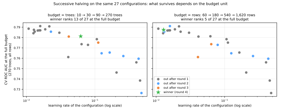
With rows as the budget, the winner ranks 5th of 27 at the full budget, 0.787 against the best 0.791: a good pick for a seventh of the cost. With trees as the budget, the winner ranks 13th (0.781), and the figure shows why. The best configurations at 270 trees all have small learning rates (0.01–0.03), and every one of them was eliminated in the first round. You saw the reason in Gradient Boosting: with a small learning rate, 10 trees have barely started, so a slow learner always looks worse early than a fast one, even when it ends better. When the budget unit interacts with a hyperparameter, the early ranking is biased, and halving eliminates the configurations it should keep. Two ways out: use a budget unit that does not interact with the knobs being searched (rows, here), or use early stopping and let the learning rate and the number of trees be tuned together.
Hyperband: several tournaments
How aggressive should the tournament be? Starting 27 configurations at 10 trees explores widely but trusts a very small budget; starting 4 configurations at the full budget trusts nothing and explores little. Hyperband (Li et al., 2018) does not choose: it runs several tournaments ("brackets") of different aggressiveness, each costing about the same. With a full budget of \(R = 27\) units and \(\eta = 3\):
R, eta = 27, 3                          # the full budget, in units of the smallest one; the factor
s_max = round(np.log(R) / np.log(eta))  # 3
for s in range(s_max, -1, -1):
    n = int(np.ceil((s_max + 1) / (s + 1) * eta ** s))     # configurations the bracket starts with
    r = R // eta ** s                                       # budget each gets in round 1
    rounds = [(n // eta ** i, r * eta ** i) for i in range(s + 1)]
    print(f"bracket s = {s}:  " + '  →  '.join(f"{ni:2d} × {ri:2d}" for ni, ri in rounds)
          + f"   cost {sum(ni * ri for ni, ri in rounds)}")
bracket s = 3:  27 ×  1  →   9 ×  3  →   3 ×  9  →   1 × 27   cost 108
bracket s = 2:  12 ×  3  →   4 ×  9  →   1 × 27   cost 99
bracket s = 1:   6 ×  9  →   2 × 27   cost 108
bracket s = 0:   4 × 27   cost 108
Bracket 3 is the aggressive tournament of the table above (27 configurations, 1 unit each). Bracket 0 is plain random search: 4 configurations at the full budget, no elimination. In between, brackets 2 and 1 hedge. Each bracket costs about 100 units, the whole thing 423 units (about 16 full evaluations) for 49 configurations. If the early ranking is reliable, bracket 3 finds the winner cheaply; if it is misleading, as with trees and learning rates above, bracket 0 still gives the slow learners a fair chance. BOHB (Falkner, Klein & Hutter, 2018) replaces Hyperband's random draws with TPE-like densities, and Optuna's HyperbandPruner brings the same idea to pruning.
Full-pipeline AutoML
Stage 5. Everything so far tuned the knobs of one or two model families. The widest form of AutoML searches the whole pipeline jointly: imputation, encoding, scaling, feature selection, the model family, its hyperparameters, and finally how to combine the best models. Thornton et al. (2013) named it the CASH problem (Combined Algorithm Selection and Hyperparameter optimization): it is the conditional space of the Optuna example, with many more branches. The main systems differ in what they search and how:
| system | what it searches | how | what it returns |
|---|---|---|---|
| auto-sklearn (Feurer et al., 2015) | 15 classifiers, 14 feature preprocessors, 4 data preprocessors: 110 hyperparameters | Bayesian optimization (a random-forest surrogate, SMAC), warm-started with configurations that worked on similar data sets (meta-learning) | an ensemble of the models found, built by ensemble selection (Caruana et al., 2004) |
| TPOT (Olson et al., 2016) | pipelines of arbitrary shape, as trees of scikit-learn steps | genetic programming: pipelines are mutated and crossed over generations | the best pipeline, exported as scikit-learn code |
| AutoGluon-Tabular (Erickson et al., 2020) | a fixed list of strong families (boosters, forests, k-NN, neural networks) with good defaults | little search: k-fold bagging of every model and stacking in several layers | a multi-layer stacked ensemble |
| FLAML (Wang et al., 2021) | boosters, forests, linear models and their hyperparameters | cost-aware search that starts from cheap configurations and moves to expensive ones only when they pay | the best single model within a time budget |
Two ideas recur. Ensembles: a search evaluates hundreds of models, and averaging the predictions of several good, different ones is usually better than the best one alone; ensemble selection greedily adds the model that most improves the validation score of the average, with replacement. Warm starts: a search that begins from configurations that worked on similar problems wastes fewer trials. The price is a very heavy tool: AutoGluon installs several gigabytes of dependencies and trains dozens of models, and auto-sklearn officially supports only Linux. Their interfaces are short; an illustrative fragment, not run here:
# AutoGluon: pip install autogluon  (heavy: several GB of dependencies)
from autogluon.tabular import TabularPredictor
predictor = TabularPredictor(label='defective', eval_metric='roc_auc').fit(
    train_df, time_limit=600, presets='best_quality')     # stacks and bags many model families
predictor.leaderboard(test_df)

# FLAML: pip install flaml
from flaml import AutoML
automl = AutoML()
automl.fit(X_dev, y_dev, task='classification', metric='roc_auc', time_budget=60)
print(automl.best_estimator, automl.best_config)
Notice what you still have to write: the label, the metric, the time limit and, before any of this, train_df and test_df. That is where the next section begins.
What AutoML cannot do
An automated search optimizes exactly the number you give it, on exactly the data you give it. Everything wrong with that number or that data, it optimizes too, and harder than a person would.
It optimizes the leak you gave it
Suppose kc1 came with one more column: bug_reports, the number of bug reports filed against each module. It is a real measurement, and it is strongly related to the target. But it is filled in after release, and the model is meant to flag risky modules before release, when the count is still zero for everyone. It is the feature that knows the future. Give the same random search both versions of the table:
from sklearn.model_selection import RandomizedSearchCV

rng = np.random.default_rng(0)


def add_bug_reports(X, y):
    """A column filled in AFTER release: bug reports filed against the module."""
    X = X.copy()
    X['bug_reports'] = rng.poisson(np.where(y == 1, 2.0, 0.3))
    return X


X_dev_leak, X_test_leak = add_bug_reports(X_dev, y_dev), add_bug_reports(X_test, y_test)
X_test_prod = X_test_leak.assign(bug_reports=0)     # at prediction time, nothing is filed yet

searches = {}
for name, X_search in [('without the column', X_dev), ('with bug_reports', X_dev_leak)]:
    searches[name] = RandomizedSearchCV(HistGradientBoostingClassifier(random_state=0), space,
                                        n_iter=20, cv=cv, scoring='roc_auc',
                                        random_state=0).fit(X_search, y_dev)
    print(f"{name:19s} best CV ROC AUC {searches[name].best_score_:.3f}")


def test_auc(search, X_):
    return roc_auc_score(y_test, search.predict_proba(X_)[:, 1])


print(f"test, honest winner:                     {test_auc(searches['without the column'], X_test):.3f}")
print(f"test, leaky winner, column filled in:    {test_auc(searches['with bug_reports'], X_test_leak):.3f}")
print(f"test, leaky winner, as it will be used:  {test_auc(searches['with bug_reports'], X_test_prod):.3f}")
without the column  best CV ROC AUC 0.792
with bug_reports    best CV ROC AUC 0.916
test, honest winner:                     0.804
test, leaky winner, column filled in:    0.962
test, leaky winner, as it will be used:  0.782
The search does its job perfectly. With the column, its best configuration reaches a CV ROC AUC of 0.916 against 0.792, and on a test set built the same way, 0.962. Every automated check passes, because every check was run on the historical table, where the column is filled in. On modules as they will actually be scored, with bug_reports = 0, the same model falls to 0.782, below the honest model's 0.804. It learned to lean on a column that will not exist, and it is worse than a model that never saw it. No search method, however clever, can catch this: the leak is in the data. The permutation importance of the finished model would show which column it leans on, but only someone who knows when each column is recorded can tell that leaning on it is illegitimate.
A longer search overfits the validation data
The winner's curse says that the best of many noisy scores is optimistic. An AutoML run is a machine for producing many noisy scores, so the curse grows with its budget. The figure runs random search on kc1 for up to 150 trials, many times over, and follows the configuration it would choose: its CV score (what the search reports) and its score on a large untouched test set (what it delivers) (figure script):
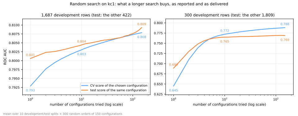
With 1,687 development rows, the search is worth running for longer and says so honestly: from 10 to 150 trials, the chosen configuration's CV score goes from 0.803 to 0.808 and its test score from 0.804 to 0.809. (The test curve starts above the CV curve because the final model is refit on all the development rows, 25% more than each CV fold trained on.) With 300 development rows, it is a different story. The first 10 trials help a lot (the first random configuration is often a poor one), but from 10 to 150 trials the reported score climbs by 0.016, from 0.772 to 0.788, while the delivered one moves by 0.004, from 0.765 to 0.769. Three quarters of the reported gain is the search fitting the quirks of 300 rows. The less data, the noisier each CV score, and the more a long search finds lucky configurations rather than good ones. Two consequences:
- Budget is not free. Past a point, more trials buy optimism, not performance. Stop when the best score has stopped moving by more than its fold standard deviation.
- Grade the whole search, not its winner. The score an AutoML tool reports for its best model carries the curse. Measure it on a locked test set, once, or wrap the entire search in an outer cross-validation (nested CV), as the lab does.
The rest of the job
What remains, even with the best search:
- Framing the problem. What is predicted, for whom, at what moment, and what an error costs. The search cannot know that a false alarm costs an engineer an hour and a missed defect costs a mission.
- Choosing the metric. The search maximizes the metric you name. On kc1, 84.5% of modules are clean, so a search on accuracy would happily approve a model that never flags anything (see Classification Metrics).
- The validation design. Groups, time order and leaks, as above. A random split of time-ordered data will be exploited by the search, not corrected by it.
- Data quality and features. An hour spent on one good feature usually beats a day of search; in Gradient Boosting, removing one leaky column changed the average precision by 0.18, and tuning by 0.007.
- Deployment and monitoring. A stacked ensemble of 40 models may be the most accurate and the hardest to serve, explain and retrain. See MLOps.
A practical default
- Lock a test set away and fix one
cv. 2. Baselines first: aDummyClassifier, a linear model, a gradient-boosting model with defaults. 3. Search the booster (log scales for everything multiplicative) with random search or Optuna, 30–100 trials; include the simple model in the space. 4. For large data or slow models, add halving or pruning, with a budget unit that does not interact with the knobs. 5. Stop when the best score stops moving by more than its fold standard deviation. 6. Report the locked test score of the winner, or a nested CV of the whole search, never the search's own best score.
Lab: four searches, one budget
The data is phoneme, from a speech-recognition project: 5,404 vowel sounds, each described by the amplitudes of its first five harmonics, and the task is to tell oral vowels from nasal ones. The model is a HistGradientBoostingClassifier with early stopping; the metric is ROC AUC. Four searches get the same budget, 27 evaluations of a 3-fold cross-validation each: a grid, random search, TPE with Optuna, and successive halving with the same number of training rows. Then the winner meets the test set once, and a nested cross-validation grades the search itself.
The lab needs Optuna, which is not preinstalled in Colab: run !pip install optuna in the first cell. Run the blocks in order, in one session; every output below is what the code prints (all together they take two to three minutes). To work on it directly, download the lab notebook and open it in Jupyter or Colab (File → Upload notebook). With another version of Optuna, the TPE numbers of step 6 may differ slightly.
Step 1 — load the vowels
# In Colab, install Optuna first:  !pip install optuna
import numpy as np
import pandas as pd
from sklearn.datasets import fetch_openml

phoneme = fetch_openml(data_id=1489, as_frame=True)    # 5,404 vowels, 5 harmonic amplitudes each
X = phoneme.data
y = (phoneme.target == '2').astype(int)                 # 1 = oral vowel, 0 = nasal vowel
print(X.shape)
print(y.value_counts())
print(X.describe().loc[['mean', 'std', 'min', 'max']].round(2))
(5404, 5)
Class
0    3818
1    1586
Name: count, dtype: int64
        V1    V2    V3    V4    V5
mean  0.00  0.00  0.00 -0.00 -0.00
std   1.00  1.00  1.00  1.00  1.00
min  -2.93 -3.04 -2.80 -2.49 -2.37
max   3.83  3.66  2.63  3.05  4.59
5,404 vowels: 1,586 oral (29%) and 3,818 nasal. The five columns are harmonic amplitudes that the data set's authors already standardized (mean 0, standard deviation 1), and a boosted model would not need scaling anyway, so there is no preprocessing step.
Step 2 — lock the test set away, fix the folds, set baselines
from sklearn.dummy import DummyClassifier
from sklearn.ensemble import HistGradientBoostingClassifier
from sklearn.linear_model import LogisticRegression
from sklearn.model_selection import StratifiedKFold, cross_val_score, train_test_split
from sklearn.pipeline import make_pipeline
from sklearn.preprocessing import StandardScaler

X_dev, X_test, y_dev, y_test = train_test_split(X, y, test_size=0.2, stratify=y, random_state=42)
cv = StratifiedKFold(n_splits=3, shuffle=True, random_state=42)     # one cv for every search


def model(**params):
    """The model every search tunes; early stopping chooses the number of trees."""
    return HistGradientBoostingClassifier(max_iter=500, early_stopping=True, n_iter_no_change=10,
                                          random_state=42, **params)


baselines = {'dummy': DummyClassifier(),
             'logistic regression': make_pipeline(StandardScaler(), LogisticRegression()),
             'boosting, defaults': model()}
baseline = {}
for name, est in baselines.items():
    s = cross_val_score(est, X_dev, y_dev, cv=cv, scoring='roc_auc')
    baseline[name] = s.mean()
    print(f"{name:20s} ROC AUC {s.mean():.4f} ± {s.std():.4f}")
dummy                ROC AUC 0.5000 ± 0.0000
logistic regression  ROC AUC 0.8195 ± 0.0154
boosting, defaults   ROC AUC 0.9468 ± 0.0042
The dummy sits at 0.5, as always for ROC AUC. The logistic regression reaches 0.8195: in these five amplitudes the two classes are far from linearly separable. The boosted model with its default settings (and early stopping) reaches 0.9468 ± 0.0042, and that is the number every search has to beat. Keep its standard deviation in mind: differences of about 0.004 between configurations are the size of the fold-to-fold noise. model() is the only estimator the searches will tune, and cv is shared by all of them, so every configuration of every method is scored on the same three folds.
Step 3 — the search space
from scipy.stats import loguniform, rv_discrete
from sklearn.model_selection import ParameterSampler


def log_int(low, high):
    """Integers from low to high, uniform on the log scale: P(k) proportional to 1/k."""
    k = np.arange(low, high + 1)
    return rv_discrete(values=(k, (1 / k) / (1 / k).sum()))


space = {'learning_rate': loguniform(0.01, 0.5),
         'max_leaf_nodes': log_int(4, 128),
         'min_samples_leaf': log_int(2, 100),
         'l2_regularization': loguniform(1e-3, 10),
         'max_features': [0.5, 0.75, 1.0]}
BUDGET = 27                                             # configurations per method, 3 fits each


def show(params):
    return ', '.join(f"{k}={v:.3g}" for k, v in sorted(params.items()))


for p in ParameterSampler(space, n_iter=4, random_state=0):
    print(show(p))
l2_regularization=0.157, learning_rate=0.164, max_features=0.75, max_leaf_nodes=33, min_samples_leaf=8
l2_regularization=0.0155, learning_rate=0.0125, max_features=0.5, max_leaf_nodes=14, min_samples_leaf=42
l2_regularization=0.13, learning_rate=0.0923, max_features=0.75, max_leaf_nodes=71, min_samples_leaf=6
l2_regularization=0.391, learning_rate=0.0422, max_features=0.75, max_leaf_nodes=58, min_samples_leaf=58
Four draws from the space. rv_discrete builds an integer distribution from a list of values and their probabilities; with probabilities proportional to \(1/k\), the range 4–8 leaves is as likely as 64–128, the log scale of Designing the search space for integers. Any object with an .rvs method can go into a scikit-learn search space. The ranges are deliberately wide: a factor of 50 in learning rate, 4 to 128 leaves, 2 to 100 rows per leaf. The number of trees is not in the space: early stopping chooses it. Each method gets BUDGET = 27 configurations, that is 81 fits of the model.
Step 4 — grid search
from sklearn.model_selection import GridSearchCV

grid = {'learning_rate': [0.03, 0.1, 0.3],
        'max_leaf_nodes': [8, 32, 128],
        'min_samples_leaf': [5, 20, 80]}                # 3 × 3 × 3 = 27 configurations
grid_search = GridSearchCV(model(), grid, cv=cv, scoring='roc_auc').fit(X_dev, y_dev)
print(f"grid:   best ROC AUC {grid_search.best_score_:.4f} · {grid_search.best_params_}")
A reasonable grid, the kind anyone would write by hand: three values of the three knobs everyone tunes. Its winner reaches 0.9498, and it sits in a corner of the grid: the largest learning rate, the most leaves and the smallest leaf size. A winner on the edge of a grid says that the grid was too narrow in that direction; to find out what lies beyond, you would have to extend it and pay for another round of evaluations.
Step 5 — random search
from sklearn.model_selection import RandomizedSearchCV

random_search = RandomizedSearchCV(model(), space, n_iter=BUDGET, cv=cv, scoring='roc_auc',
                                   random_state=0).fit(X_dev, y_dev)
print(f"random: best ROC AUC {random_search.best_score_:.4f} · {show(random_search.best_params_)}")
random: best ROC AUC 0.9499 · l2_regularization=8.21, learning_rate=0.228, max_features=0.75, max_leaf_nodes=58, min_samples_leaf=2
Random search reaches 0.9499, a tie with the grid, with a configuration no hand-made grid would contain (a leaf size of 2, an L2 penalty of 8.21, 75% of the features per split), and it explored five knobs for the price the grid paid for three.
Step 6 — TPE with Optuna
import optuna
optuna.logging.set_verbosity(optuna.logging.WARNING)


def objective(trial):
    params = {'learning_rate': trial.suggest_float('learning_rate', 0.01, 0.5, log=True),
              'max_leaf_nodes': trial.suggest_int('max_leaf_nodes', 4, 128, log=True),
              'min_samples_leaf': trial.suggest_int('min_samples_leaf', 2, 100, log=True),
              'l2_regularization': trial.suggest_float('l2_regularization', 1e-3, 10, log=True),
              'max_features': trial.suggest_categorical('max_features', [0.5, 0.75, 1.0])}
    return cross_val_score(model(**params), X_dev, y_dev, cv=cv, scoring='roc_auc').mean()


study = optuna.create_study(direction='maximize', sampler=optuna.samplers.TPESampler(seed=0))
study.optimize(objective, n_trials=BUDGET)
print(f"TPE:    best ROC AUC {study.best_value:.4f} · {show(study.best_params)}")
TPE: best ROC AUC 0.9510 · l2_regularization=1.23, learning_rate=0.189, max_features=1, max_leaf_nodes=102, min_samples_leaf=2
TPE reaches 0.9510 with 102 leaves and leaves of 2 rows: the direction of the grid's corner (big trees, small leaves), found by learning rather than by enumeration. The space is written again in Optuna's words; log=True plays the role of loguniform and log_int.
Step 7 — successive halving, same budget in rows
from sklearn.experimental import enable_halving_search_cv  # noqa: F401
from sklearn.model_selection import HalvingRandomSearchCV

halving = HalvingRandomSearchCV(model(), space, n_candidates=180, factor=3, min_resources=160,
                                cv=cv, scoring='roc_auc', random_state=1).fit(X_dev, y_dev)
rows = sum(n * r for n, r in zip(halving.n_candidates_, halving.n_resources_))
print('candidates per round:', halving.n_candidates_)
print('rows per candidate:  ', halving.n_resources_)
print(f"budget in rows: halving {rows:,} · random search {BUDGET * len(X_dev):,}")
print(f"fits:           halving {3 * sum(halving.n_candidates_)} · random search {3 * BUDGET}")
print(f"halving: best ROC AUC {halving.best_score_:.4f} · {show(halving.best_params_)}")
candidates per round: [180, 60, 20, 7]
rows per candidate:   [160, 480, 1440, 4320]
budget in rows: halving 116,640 · random search 116,721
fits:           halving 801 · random search 81
halving: best ROC AUC 0.9528 · l2_regularization=2.75, learning_rate=0.0823, max_features=0.5, max_leaf_nodes=114, min_samples_leaf=5
The tournament starts 180 candidates on 160 rows each (with 3-fold CV, each fit trains on about 107 rows), keeps 60 for 480 rows, 20 for 1,440, and 7 for 4,320, almost all of the 4,323 development rows. In rows, the budget is the same as random search's: 116,640 against 116,721. In fits, it is not: 801 against 81. Hundreds of tiny fits each carry a fixed cost (binning the features, setting up early stopping), so equal rows do not mean equal time: on the machine used for this page, the grid, random search and TPE took about 20 seconds each, and halving about 45. For that price, halving looked at 180 configurations instead of 27, and found the best CV score of the four methods, 0.9528 (114 leaves, leaf size 5, learning rate 0.082).
Step 8 — the best score so far, evaluation by evaluation
import matplotlib.pyplot as plt

runs = {'grid': grid_search.cv_results_['mean_test_score'],
        'random': random_search.cv_results_['mean_test_score'],
        'TPE': [t.value for t in study.trials]}
best_so_far = pd.DataFrame({name: np.maximum.accumulate(v) for name, v in runs.items()},
                           index=pd.RangeIndex(1, BUDGET + 1, name='evaluations'))
print(best_so_far.loc[[1, 5, 10, 15, 20, 27]].round(4))
print(f"halving, same budget in rows: {halving.best_score_:.4f}")

ax = best_so_far.plot(drawstyle='steps-post', figsize=(7, 3.5))
ax.axhline(halving.best_score_, color='gray', ls='--', label='halving (same budget)')
ax.axhline(baseline['boosting, defaults'], color='gray', ls=':', label='defaults')
ax.set_ylabel('best CV ROC AUC so far')
ax.legend()
plt.show()
               grid  random     TPE
evaluations
1            0.9327  0.9475  0.9476
5            0.9464  0.9499  0.9489
10           0.9465  0.9499  0.9489
15           0.9467  0.9499  0.9510
20           0.9496  0.9499  0.9510
27           0.9498  0.9499  0.9510
halving, same budget in rows: 0.9528
(figure script; it reruns the lab, plus random search and TPE with four more seeds)
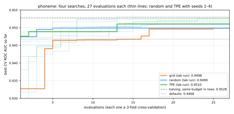
Read the table row by row. After one evaluation the grid is at 0.9327: it lists its configurations in a fixed order, and the first one (learning rate 0.03, 8 leaves) is slow and small. Random search and TPE start with a random draw, at 0.9475. Random search found its best configuration by the fifth evaluation and never improved on it. TPE's first 10 trials are random too (0.9489 after 10), and its guided trials found 0.9510 before the fifteenth. The grid lists its cells with the learning rate changing slowest, so its first 128-leaf cell with a learning rate of 0.1 came only at evaluation 16, and it reached 0.9496 at evaluation 17. Its cv_results_ also show where the budget went: the nine 8-leaf cells all scored between 0.931 and 0.937, whatever the learning rate. The knob that mattered most here, the number of leaves, got only three values, and a third of the grid was spent on its worst one: Bergstra & Bengio's argument, on real data.
Now the thin lines of the figure. With four other seeds, random search ends between 0.9512 and 0.9522 and TPE between 0.9519 and 0.9532: the lab's run (seed 0) was the unluckiest of the five for both. Seed by seed, TPE finishes ahead in 4 of the 5 runs, by 0.001 on average, which is smaller than the spread between seeds of one method and a quarter of the fold standard deviation. Halving's 0.9528 falls inside TPE's range. On this problem, then, the space (big trees, small leaves) matters more than the method, and every method gains 0.003 to 0.006 over the defaults, about one fold standard deviation.
Step 9 — the one and only test
from sklearn.metrics import roc_auc_score

winners = {'grid': (grid_search.best_score_, grid_search.best_params_),
           'random': (random_search.best_score_, random_search.best_params_),
           'TPE': (study.best_value, study.best_params),
           'halving': (halving.best_score_, halving.best_params_)}
name = max(winners, key=lambda k: winners[k][0])        # the rule: best CV score, decided in advance
cv_score, params = winners[name]
final = model(**params).fit(X_dev, y_dev)
print(f"chosen: the {name} winner · {show(params)}")
print(f"chosen:   CV ROC AUC {cv_score:.4f} · test ROC AUC "
      f"{roc_auc_score(y_test, final.predict_proba(X_test)[:, 1]):.4f}")

reference = model().fit(X_dev, y_dev)                   # not a candidate: the choice is made
print(f"defaults: CV ROC AUC {baseline['boosting, defaults']:.4f} · test ROC AUC "
      f"{roc_auc_score(y_test, reference.predict_proba(X_test)[:, 1]):.4f}")
chosen: the halving winner · l2_regularization=2.75, learning_rate=0.0823, max_features=0.5, max_leaf_nodes=114, min_samples_leaf=5
chosen:   CV ROC AUC 0.9528 · test ROC AUC 0.9455
defaults: CV ROC AUC 0.9468 · test ROC AUC 0.9374
The rule was fixed before looking: the configuration with the best CV score, whichever method found it. That is the halving winner, chosen among 27 + 27 + 27 + 180 = 261 configurations. On the test set it scores 0.9455, 0.007 below its CV score. Is that the winner's curse? The untuned defaults, scored on the same test set only as a reference (they were not a candidate, and nothing is chosen from this line), drop by about as much, from 0.9468 to 0.9374: these 1,081 test rows are simply a little harder than the development folds. Measured against the defaults on the same rows, tuning is worth +0.008 on the test set, in line with the +0.006 it showed in cross-validation.
Step 10 — an honest estimate of the search
outer = StratifiedKFold(n_splits=3, shuffle=True, random_state=7)
nested = cross_val_score(random_search, X_dev, y_dev, cv=outer, scoring='roc_auc')
print(f"random search, best_score_:     {random_search.best_score_:.4f}")
print(f"random search, nested estimate: {nested.mean():.4f} ± {nested.std():.4f}  {nested.round(4)}")
random search, best_score_:     0.9499
random search, nested estimate: 0.9472 ± 0.0067  [0.9463 0.9394 0.9558]
cross_val_score accepts the search object as if it were a model: in each of the 3 outer folds it runs the whole random search (27 configurations × 3 inner folds) on the outer training part and grades the configuration it picks on the outer validation part, which the search never saw. This is the nested CV of the cross-validation lesson, applied to a search. The honest estimate of "random search with 27 trials" is 0.9472 ± 0.0067, below the 0.9499 that the search reported for itself: 0.003 of optimism, the same size as the whole gain of the search over the defaults (0.9468). The outer folds range from 0.9394 to 0.9558, a spread far larger than the differences between the four methods. On phoneme, a tuned model is a little better than the defaults, and the only numbers that say by how much are the ones measured on data the search never touched.
Your turn
- Luck of the seed. Rerun steps 5 and 6 with
random_state=1, 2, 3, 4andTPESampler(seed=1, 2, 3, 4). Tabulate the best score of each run. Is the gap between TPE and random search larger than the spread between seeds of the same method? What does that say about declaring a winner from one run of each? - Prune. Rewrite the objective of step 6 as a loop over the folds of
cv, withtrial.reportandtrial.should_prune(), and create the study withpruner=optuna.pruners.MedianPruner(n_startup_trials=5, n_warmup_steps=1)(the kc1 example in Pruning shows how). Run 60 trials. How many were pruned, how many folds were fitted, and did the best score change? - Two families. Add a branch to the objective,
family = trial.suggest_categorical('family', ['boosting', 'svm']), where the SVM ismake_pipeline(StandardScaler(), SVC(C=..., gamma=...))withCandgammaon log scales (usedecision_functionscores, orcross_val_scorewithscoring='roc_auc', which handles it). How many of 40 trials does TPE give each family, and which one wins? - The wrong budget unit. Rerun step 7 with the number of trees as the budget:
model()withearly_stopping=False, andresource='max_iter', min_resources=10, max_resources=270, n_candidates=27. Which learning rates survive to the last round? Score the winner with 270 trees and compare it with step 7's winner, as in What the tournament assumes.
Class materials
Lab notebook
The lab of this lesson as a notebook, ready for Jupyter or Colab: lab notebook. In Colab, run !pip install optuna first.
References
- Bergstra, J.; Bengio, Y. "Random Search for Hyper-Parameter Optimization." JMLR 13 (2012): 281–305 — random against grid search, and the low effective dimensionality of tuning problems. full text
- Jones, D. R.; Schonlau, M.; Welch, W. J. "Efficient Global Optimization of Expensive Black-Box Functions." Journal of Global Optimization 13 (1998): 455–492 — a Gaussian-process surrogate and the expected improvement. DOI
- Snoek, J.; Larochelle, H.; Adams, R. P. "Practical Bayesian Optimization of Machine Learning Algorithms." NeurIPS 25 (2012): 2951–2959 — Bayesian optimization applied to tuning machine-learning models. arXiv:1206.2944
- Bergstra, J.; Bardenet, R.; Bengio, Y.; Kégl, B. "Algorithms for Hyper-Parameter Optimization." NeurIPS 24 (2011): 2546–2554 — the Tree-structured Parzen Estimator (TPE). full text
- Akiba, T.; Sano, S.; Yanase, T.; Ohta, T.; Koyama, M. "Optuna: A Next-generation Hyperparameter Optimization Framework." KDD '19 (2019): 2623–2631 — define-by-run search spaces and pruning. DOI
- Jamieson, K.; Talwalkar, A. "Non-stochastic Best Arm Identification and Hyperparameter Optimization." AISTATS, PMLR 51 (2016): 240–248 — successive halving for hyperparameter search. full text
- Li, L.; Jamieson, K.; DeSalvo, G.; Rostamizadeh, A.; Talwalkar, A. "Hyperband: A Novel Bandit-Based Approach to Hyperparameter Optimization." JMLR 18, no. 185 (2018): 1–52. full text
- Falkner, S.; Klein, A.; Hutter, F. "BOHB: Robust and Efficient Hyperparameter Optimization at Scale." ICML, PMLR 80 (2018): 1437–1446 — Hyperband with a TPE-like model. full text
- Thornton, C.; Hutter, F.; Hoos, H. H.; Leyton-Brown, K. "Auto-WEKA: Combined Selection and Hyperparameter Optimization of Classification Algorithms." KDD '13 (2013): 847–855 — the CASH problem. DOI
- Feurer, M.; Klein, A.; Eggensperger, K.; Springenberg, J.; Blum, M.; Hutter, F. "Efficient and Robust Automated Machine Learning." NeurIPS 28 (2015): 2962–2970 — auto-sklearn. full text
- Caruana, R.; Niculescu-Mizil, A.; Crew, G.; Ksikes, A. "Ensemble Selection from Libraries of Models." ICML (2004) — the greedy ensemble used by auto-sklearn. DOI
- Olson, R. S.; Bartley, N.; Urbanowicz, R. J.; Moore, J. H. "Evaluation of a Tree-based Pipeline Optimization Tool for Automating Data Science." GECCO '16 (2016): 485–492 — TPOT. DOI
- Erickson, N.; Mueller, J.; Shirkov, A.; Zhang, H.; Larroy, P.; Li, M.; Smola, A. "AutoGluon-Tabular: Robust and Accurate AutoML for Structured Data." (2020). arXiv:2003.06505
- Wang, C.; Wu, Q.; Weimer, M.; Zhu, E. "FLAML: A Fast and Lightweight AutoML Library." MLSys 3 (2021). arXiv:1911.04706
- Hutter, F.; Kotthoff, L.; Vanschoren, J. (eds.) Automated Machine Learning: Methods, Systems, Challenges. Springer (2019) — the open-access reference book of the field. DOI
- Sayyad Shirabad, J.; Menzies, T. J. The PROMISE Repository of Software Engineering Databases. University of Ottawa (2005) — the kc1 data used in this lesson (OpenML 1067).
- Phoneme data set, from the ESPRIT 5516 ROARS speech-recognition project, distributed by the ELENA project — the lab data (OpenML 1489).
- Optuna — hyperparameter optimization.