The question no lesson asked yet
- Every model comes with knobs; Model Selection explained what they do, Cross-Validation how to compare the results honestly.
- A grid with 5 hyperparameters and 5 values each: 3,125 cross-validations, most of them in regions that were obviously bad after the first dozen.
hyperparameter optimization
treats the search itself as an optimization problem
AutoML
pushes the same idea to the whole pipeline: preprocessing, family, hyperparameters, the final ensemble
The path of this lesson
- Frame the searchan expensive, noisy black box; the search space
- Grid or randomBergstra & Bengio, measured
- A search that learnsBayesian optimization, TPE, Optuna
- Stop bad trials earlypruning, successive halving, Hyperband
- Automate, then checkthe whole pipeline, leaks, a flattering score
One call to the black box
\(\lambda\): a configuration. \(f(\lambda)\): its cross-validated score. Tuning = find the \(\lambda\) with the largest \(f(\lambda)\).
- kc1: 2,109 software modules of a NASA flight system, 21 code metrics; target: was a defect found later? (15.5% defective)
- One call = a 5-fold CV ROC AUC of a boosted model.
Expensive, noisy, and a black box
| settings | 5 fold shuffles | mean |
|---|---|---|
| defaults | 0.760 · 0.776 · 0.767 · 0.769 · 0.769 | 0.768 |
| small, slow trees | 0.795 · 0.806 · 0.804 · 0.803 · 0.805 | 0.803 |
expensive
each call is 5 fits; on a real project, minutes or hours. The number of calls is the budget.
noisy
0.760 to 0.776 for the same settings: a difference of 0.01 may not be real
black box
no gradient with respect to min_samples_leaf; integers, categories, conditional knobs
Designing the space (1): the scale
| learning rate in | uniform | log-uniform |
|---|---|---|
| [0.001, 0.01) | 0.9% | 33.5% |
| [0.01, 0.1) | 9.1% | 33.2% |
| [0.1, 1) | 90.0% | 33.3% |
By hand: \(0.009 / 0.999 = 0.9\%\); on the log scale each of the 3 decades gets a third.
C, alpha, numbers of leaves or neighbors) gets a log scale: loguniform, or log=True in Optuna.Designing the space (2): conditional knobs
Cbelongs to the logistic regression,max_leaf_nodesto the booster,gammato an RBF kernel.- One grid over all of them would pair every
Cwith every tree size: the same logistic regression, fitted again and again.
if.Grid or random? The argument
- A score that depends on one hyperparameter \(x_1\) (a bump of width 0.05); the other \(d - 1\) do nothing.
- A grid with \(k\) values per axis costs \(k^d\) evaluations, but tries \(x_1\) at only \(k\) values.
- Random search with budget \(B\) tries \(x_1\) at \(B\) values, whatever \(d\) is.
Grid or random? Measured on 4,000 problems
| d | budget | grid | random |
|---|---|---|---|
| 2 | 9 | 0.378 | 0.629 |
| 2 | 81 | 0.824 | 0.985 |
| 3 | 27 | 0.378 | 0.900 |
| 4 | 81 | 0.378 | 0.986 |
| 4 | 256 | 0.501 | 0.998 |
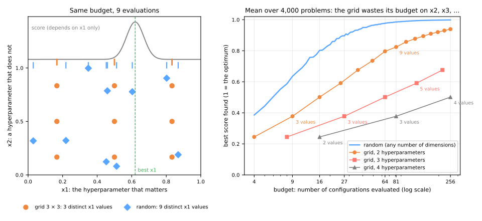
Mean best score. The grid pays for every irrelevant axis with a multiplication of its cost; random search pays nothing (Bergstra & Bengio, 2012).
Simulator: same budget, different searches
Predict. Budget 81: how many distinct values of \(x_1\) does the 9 × 9 grid try, and how many does random search try?
Bayesian optimization: a search that learns
Random search draws the 27th configuration exactly like the first. When each evaluation costs an hour, that is wasteful.
- fit a cheap surrogate to the (configuration, score) pairs so far: it predicts the score anywhere, with an uncertainty;
- choose the next configuration by maximizing an acquisition function: exploitation (high predicted score) against exploration (high uncertainty);
- evaluate it, add it to the history, repeat.
A stand-in score with a known truth: a broad peak of 0.78 at 0.25 and a higher, narrower one of 0.82 at 0.72.
The surrogate: a Gaussian process
Three evaluations so far: 0.15 and 0.35 (0.72943), 0.95 (0.700). Best so far \(f^+ = 0.72943\).
| \(x\) | mean \(\mu\) | sd \(\sigma\) | reading |
|---|---|---|---|
| 0.25 | 0.73076 | 0.00419 | between two points: nearly sure, just above \(f^+\) |
| 0.55 | 0.72212 | 0.01246 | far from any point: below \(f^+\), three times more uncertain |
| 0.72 | 0.71390 | 0.01318 | the real peak, but the surrogate knows nothing about it |
Expected improvement, by hand
\[ \mathrm{EI}(x) = \underbrace{(\mu - f^+)\,\Phi(z)}_{\text{exploitation}} + \underbrace{\sigma\,\varphi(z)}_{\text{exploration}}, \qquad z = \frac{\mu - f^+}{\sigma} \]| \(x\) | \(z\) | \((\mu - f^+)\Phi(z)\) | \(\sigma\varphi(z)\) | EI |
|---|---|---|---|---|
| 0.25 | +0.32 | +0.00083 | 0.00159 | 0.00242 |
| 0.55 | −0.59 | −0.00203 | 0.00417 | 0.00214 |
| 0.72 | −1.18 | −0.00185 | 0.00262 | 0.00077 |
Four iterations
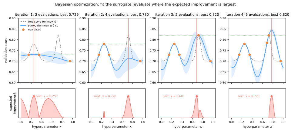
1: exploits 0.25 → 0.780. 2: its EI collapses, so it explores the gap → 0.72, 0.820. 3–4: refine at 0.685 and 0.775. Random search would need about 28 draws to land that close to 0.72.
The surrogate's assumptions matter
100 runs from random starting triples, 30 evaluations each. Share of runs that reached 0.81:
| within 10 | within 20 | within 30 | |
|---|---|---|---|
| BO, length scale 0.15 | 40% | 65% | 65% |
| BO, length scale 0.10 | 61% | 92% | 92% |
| random search | 37% | 54% | 65% |
TPE: model \(x\) given the score
- Split the trials into the good ones (best fraction \(\gamma\)) and the rest.
- Density of the good values \(\ell(x)\), density of the others \(g(x)\): one Gaussian bump per trial.
- Sample where \(\ell(x)/g(x)\) is largest (Bergstra et al., 2011).
| \(x\) | 0.1 | 0.25 | 0.5 | 0.7 | 0.9 |
|---|---|---|---|---|---|
| \(\ell / g\) | 0.03 | 1.24 | 0.45 | 5.73 | 0.09 |
Optuna: TPE against random, measured
Six hyperparameters: one matters a lot, one a little, four not at all. Best possible: 0.870. 20 seeds.
| mean best after | 10 | 20 | 40 | 60 trials |
|---|---|---|---|---|
| random | 0.812 | 0.819 | 0.830 | 0.843 |
| TPE | 0.812 | 0.847 | 0.857 | 0.860 |
Identical at 10: TPE's first 10 trials are random. After 40 it is above what random reaches after 60.
Define-by-run: the space is code
def build(trial):
    family = trial.suggest_categorical('family', ['logistic', 'boosting'])
    if family == 'logistic':
        C = trial.suggest_float('C', 1e-3, 1e2, log=True)
        return make_pipeline(FunctionTransformer(np.log1p), StandardScaler(),
                             LogisticRegression(C=C, max_iter=2000))
    return HistGradientBoostingClassifier(
        learning_rate=trial.suggest_float('learning_rate', 0.01, 0.5, log=True), ...)
C ≈ 0.03, 0.798, tied with the hand-picked booster; TPE spent 31 of its 40 trials on it. A space that leaves out the simple model can never tell you that you did not need the complicated one.Pruning: stop a bad trial early
- The objective reports its running mean after every fold (
trial.report). - The median pruner stops a trial worse than the median of earlier trials at the same fold.
Successive halving: a tournament
Start \(n = 27\) configurations on a small budget; keep the best third; give the survivors 3 × more; repeat.
| round | configurations | trees each | cost |
|---|---|---|---|
| 1 | 27 | 10 | 270 |
| 2 | 9 | 30 | 270 |
| 3 | 3 | 90 | 270 |
| 4 | 1 | 270 | 270 |
| total | 1,080 |
HalvingRandomSearchCV).What the tournament assumes
The ranking after a small budget predicts the ranking after the full one. Two tournaments: budget in trees, budget in rows.
| winner with budget | full score | rank |
|---|---|---|
| trees | 0.781 | 13 of 27 |
| rows | 0.787 | 5 of 27 |
| best at full budget | 0.791 | 1 |
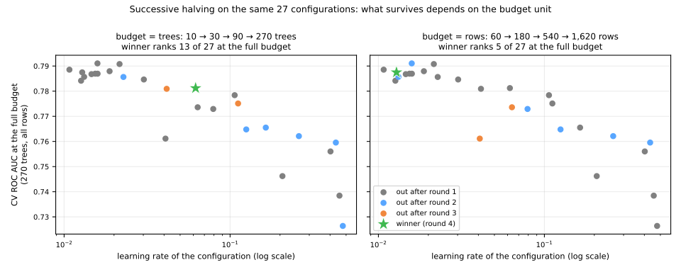
With a small learning rate, 10 trees have barely started: the slow learners, best at 270 trees, all died in round 1.
Hyperband: several tournaments
How aggressive should the tournament be? Hyperband runs brackets of different aggressiveness, each costing about the same (Li et al., 2018).
| bracket | rounds (configurations × budget) | cost |
|---|---|---|
| s = 3 | 27 × 1 → 9 × 3 → 3 × 9 → 1 × 27 | 108 |
| s = 2 | 12 × 3 → 4 × 9 → 1 × 27 | 99 |
| s = 1 | 6 × 9 → 2 × 27 | 108 |
| s = 0 | 4 × 27 (plain random search) | 108 |
Full-pipeline AutoML: the CASH problem
Combined Algorithm Selection and Hyperparameter optimization (Thornton et al., 2013).
| system | how it searches | what it returns |
|---|---|---|
| auto-sklearn | Bayesian optimization, warm-started on similar data sets | an ensemble (ensemble selection) |
| TPOT | genetic programming over pipeline trees | the best pipeline, as scikit-learn code |
| AutoGluon-Tabular | little search: bagging and multi-layer stacking | a stacked ensemble |
| FLAML | cost-aware: cheap configurations first | the best single model in a time budget |
It optimizes the leak you gave it
bug_reports: filed after release; the model must flag risky modules before release, when the count is zero for everyone.
| ROC AUC | |
|---|---|
| best CV, without the column / with it | 0.792 / 0.916 |
| test, leaky winner, column filled in | 0.962 |
| test, honest winner | 0.804 |
test, leaky winner, as it will be used (bug_reports = 0) | 0.782 |
Every automated check passes. The leak is in the data: only someone who knows when each column is recorded can catch it.
A longer search overfits the validation data
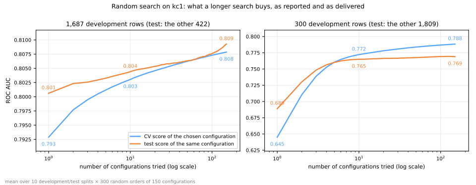
1,687 rows, 10 → 150 trials: CV 0.803 → 0.808, test 0.804 → 0.809. Honest.
300 rows: CV 0.772 → 0.788, test 0.765 → 0.769. Three quarters of the reported gain is luck.
The rest of the job
framing the problem
what is predicted, for whom, when, and what an error costs
choosing the metric
84.5% of kc1 modules are clean: a search on accuracy approves a model that never flags
the validation design
groups, time order and leaks are exploited by the search, not corrected
data and features
removing one leaky column changed average precision by 0.18; tuning, by 0.007
And deployment: a stacked ensemble of 40 models may be the hardest to serve, explain and retrain.
A practical default
- Lock a test set away and fix one
cv. - Baselines first: a dummy, a linear model, a booster with defaults.
- Random search or Optuna, 30–100 trials, log scales, the simple model in the space.
- For large data or slow models: halving or pruning, with a budget unit that does not interact with the knobs.
- Stop when the best score stops moving by more than its fold standard deviation.
- Report the locked test score, or a nested CV of the whole search, never the search's own best score.
Four searches, one budget
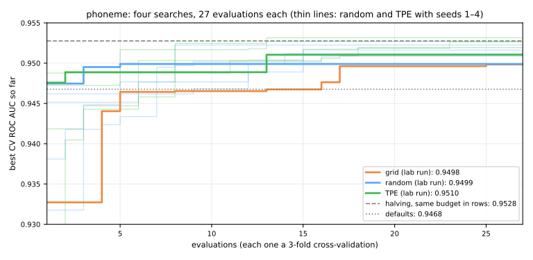
phoneme: 5,404 vowels, oral or nasal. Grid, random, TPE and halving get 27 evaluations each.
Chosen (best CV): the halving winner, CV 0.9528, test 0.9455; the defaults drop as much (0.9468 → 0.9374).
Random search: best_score_ 0.9499; nested estimate 0.9472 ± 0.0067.
Run !pip install optuna first. Lab notebook (Jupyter or Colab, File → Upload notebook).
Summary
- Tuning is an expensive, noisy black box: the budget is the number of calls.
- Design the space: log scales and conditional knobs.
- Random beats grid when only a few knobs matter.
- Bayesian optimization and TPE learn where to look; their assumptions matter.
- Halving and Hyperband stop bad configurations early, if the early ranking is right.
- A search optimizes your leaks and its own luck: grade it on untouched data.