The path of this part
- Weigh the errorsF-beta: β says how much more recall matters
- When positives are rareprevalence moves precision; balanced accuracy and MCC (Matthews correlation coefficient) resist
- Many classesone-vs-rest, then a macro, weighted or micro average
- Grade the probabilitylog loss, Brier score, calibration
Each stage answers one question: what if one mistake costs more? → which metrics survive a rare class? → how do many classes become one number? → is the probability itself right?
Stage 1 · What if one mistake costs more?
F-beta: making the trade explicit
\[ F_\beta = \frac{(1 + \beta^2)\,P \cdot R}{\beta^2 P + R} = \frac{(1 + \beta^2)\,TP}{(1 + \beta^2)\,TP + \beta^2\,FN + FP} \]The count form shows the mechanism: a miss weighs \(\beta^2\) times a false alarm.
| meaning | on the 20 patients | |
|---|---|---|
| \(F_{0.5}\) | a false alarm weighs 4× a miss | 0.761 |
| \(F_1\) | both weigh the same | 0.737 |
| \(F_2\) | a miss weighs 4× a false alarm | 0.714 |
\(P\) = precision, \(R\) = recall; TP, FP, FN and TN = true positives, false positives, false negatives and true negatives. Use F2 for screening and F0.5 when alarms are expensive. Choosing \(\beta\) is a statement about costs.
\(\beta\) moves the operating point
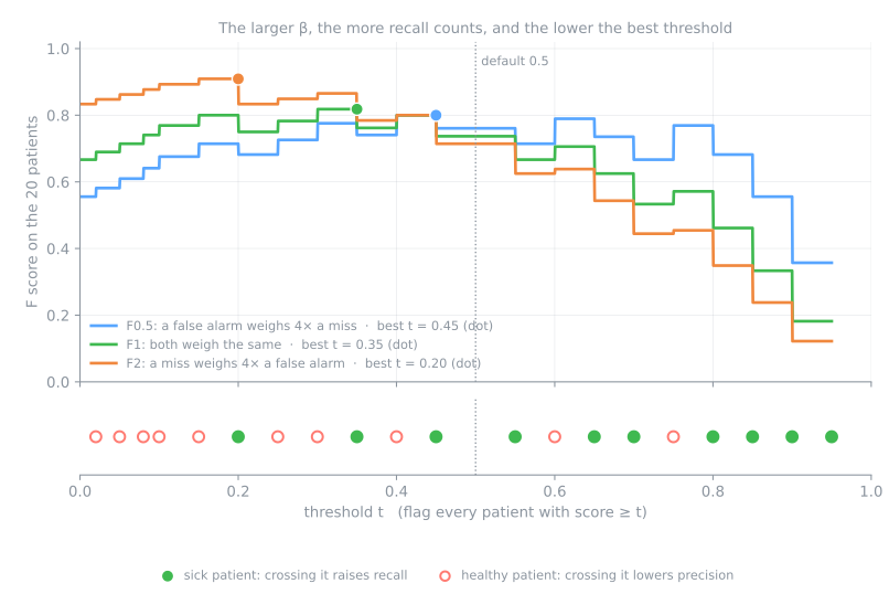
How to read it
- x axis: the threshold \(t\); the strip below shows the 20 patients at their scores;
- each step: the threshold crosses a patient. A sick one (●) raises recall; a healthy one (○) lowers precision;
- y axis: the value of F0.5, F1 and F2 at that threshold;
- dot: the threshold that maximizes each one.
The larger \(\beta\), the more recall counts and the lower the best threshold: 0.45 (F0.5) → 0.35 (F1) → 0.20 (F2). The metric you maximize picks the threshold.
Stage 2 · Which metrics survive a rare class?
Prevalence changes precision
The same model (sensitivity 0.70, specificity 0.80) on 10,000 people; NPV = negative predictive value:
| prevalence | TP | FP | precision | NPV | accuracy |
|---|---|---|---|---|---|
| 50% | 3500 | 1000 | 0.778 | 0.727 | 0.750 |
| 10% | 700 | 1800 | 0.280 | 0.960 | 0.790 |
| 1% | 70 | 1980 | 0.034 | 0.996 | 0.799 |
At 1%: of every 30 people flagged, 29 are healthy — with exactly the model that had precision 0.778 in the specialist's office.
Why some metrics do not move
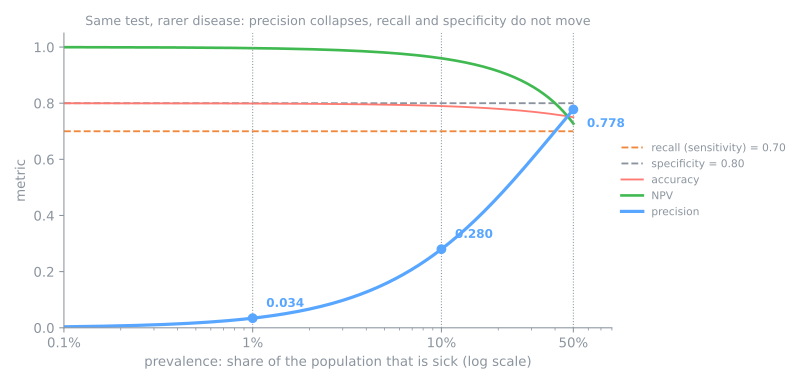
- Recall uses only the sick row and specificity only the healthy row: they are proportions within a class, so they do not depend on class sizes — the horizontal lines.
- Precision, NPV and accuracy mix the two rows, and so they move.
When reporting precision, report the prevalence of the data it was measured on. F1 inherits the same dependence.
Metrics that survive imbalance
\[ \text{balanced accuracy} = \frac{\text{recall} + \text{specificity}}{2} \qquad \text{MCC} = \frac{TP \cdot TN - FP \cdot FN}{\sqrt{(TP{+}FP)(TP{+}FN)(TN{+}FP)(TN{+}FN)}} \]| accuracy | balanced | MCC | Cohen's kappa | |
|---|---|---|---|---|
| 20 patients | 0.750 | 0.750 | 0.503 | 0.500 |
| lazy model | 0.985 | 0.745 | 0.401 | 0.393 |
| always "healthy" | 0.990 | 0.500 | 0.000 | 0.000 |
Accuracy puts the constant answer first. The other three unmask it: MCC (Matthews correlation coefficient) uses all four cells and is only high if the model does well in all of them.
Stage 3 · How do many classes become one number?
Multiclass: the matrix grows
| true \ pred. | low | medium | high |
|---|---|---|---|
| low | 110 | 9 | 1 |
| medium | 8 | 46 | 6 |
| high | 2 | 8 | 10 |
200 patients triaged into low, medium and high risk.
Precision and recall are computed per class, one-vs-rest. For high:
- TP = 10 (the diagonal)
- FN = 2 + 8 = 10 (the rest of the row)
- FP = 1 + 6 = 7 (the rest of the column)
Half the high-risk patients — exactly the ones the triage exists for — are sent to a lower level.
Three ways to get one number
| class | F1 | support |
|---|---|---|
| low | 0.917 | 120 |
| medium | 0.748 | 60 |
| high | 0.541 | 20 |
- macro = 0.735 · each class counts equally
- weighted = 0.828 · weighted by support
- micro = 0.830 = accuracy
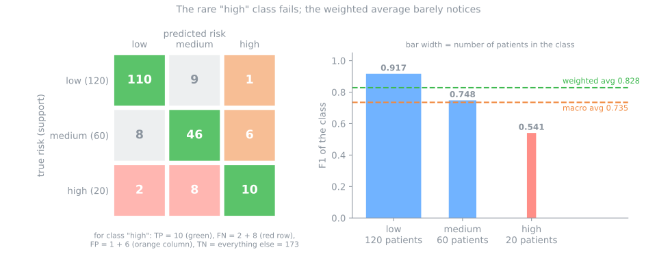
When the rare class is the important one, report macro-F1 and per-class recall: the weighted and micro averages follow the big classes.
Stage 4 · Is the probability itself right?
Grading the probability, not the label
\[ \text{log loss} = -\frac{1}{n}\sum_i \big[ y_i \ln p_i + (1 - y_i)\ln(1 - p_i) \big] \qquad \text{Brier} = \frac{1}{n}\sum_i (p_i - y_i)^2 \]| patient | score | sick | log loss | Brier |
|---|---|---|---|---|
| P01 | 0.95 | 1 | 0.051 | 0.0025 |
| P05 | 0.75 | 0 | 1.386 | 0.5625 |
| P15 | 0.20 | 1 | 1.609 | 0.64 |
In both, lower is better. A confident right answer costs almost nothing; a confident wrong one costs a lot — and log loss punishes it far more than Brier, because \(-\ln p\) grows without bound.
Same labels, worse probabilities
A second model makes the same decisions at 0.5, but declares every probability as 0.99 or 0.01:
| model | accuracy | precision | F1 | log loss | Brier |
|---|---|---|---|---|---|
| original | 0.75 | 0.778 | 0.737 | 0.463 | 0.157 |
| bold (0.99 / 0.01) | 0.75 | 0.778 | 0.737 | 1.159 | 0.245 |
Same confusion matrix, so every label metric is blind to the difference. The five mistakes, now declared with 99% confidence, cost \(-\ln 0.01 = 4.6\) each.
The neighboring question is calibration: among the patients the model calls "70%", are about 70% actually sick?
How to choose a metric
| scenario | the expensive mistake | track |
|---|---|---|
| cancer screening | FN: an undetected tumour | recall, F2 |
| confirmatory test before surgery | FP: treating a healthy person | precision, specificity |
| spam filter | FP: a real email lost | precision, F0.5 |
| ruling out a disease and sending home | FN: a sick patient released | NPV, recall |
| an imbalanced binary benchmark | any | MCC or balanced accuracy |
| multiclass with an important rare class | failing the rare class | macro-F1 and per-class recall |
| probabilities used as numbers | wrong probabilities | log loss, Brier, calibration |
There is no best metric, only the one that matches the cost of your problem's mistakes. Decide before training and record the choice.
Advanced lab · about 30 min, in pairs
Probabilities, threshold and multiclass: steps 8 to 11
- Same Colab notebook, from step 8 (Passo 8). New session? Runtime → Run before.
- Step 8: log loss sinks k-NN (1.290, worse than the baseline); simulation: does a larger k fix the probabilities?
- Step 9: the threshold on validation; simulation: β picks the threshold.
- Steps 10 and 11: the test set touched once, and a multiclass report.
Pace: steps 8 and 9 in 15 min; 10 and 11 in 10 min; wrap-up in 5 min.