Decision Trees
The models of the last lessons each draw a boundary in their own way: logistic regression and the linear SVM with a weighted sum of all the features, k-NN by distances to stored examples. A decision tree does something a person can follow with a pencil: it asks one question about one feature at a time — is the monthly bill above R$ 82.50? has the customer been with us for more than 15 months? — and walks from the root to a leaf, where the answer waits. Formalized in the 1980s (CART: Breiman et al., 1984; ID3: Quinlan, 1986), trees read like the flowcharts a domain expert already uses, need no feature scaling, and are the building block of the ensembles that dominate tabular machine learning today: random forests (next lesson) and gradient boosting.
This lesson grows a tree by hand on a 12-row table, then lets scikit-learn confirm every number: impurity, the choice of each split, the leaf probabilities, the pruning sequence. It then measures, on a real dataset, the three things you must know before using a single tree: it overfits unless stopped, it is unstable, and its boundaries are axis-aligned staircases. Every number quoted comes from the code blocks or from the figure scripts next to this page.
How this lesson is organized
The lesson has two approaches. Each has slides, text and a lab to do in class on Colab; the quiz at the end covers the fundamental one. Start with the fundamental approach: the advanced one builds on it.
| Fundamental approach | Advanced approach | |
|---|---|---|
| question | How does a tree choose its questions, how does it answer, and why must it be stopped? | Where trees shine, where they fail, and why they became the raw material of ensembles |
| content | the parts of a tree, Gini and entropy, the search for the best split, greedy recursive growth, leaves and probabilities, overfitting and pre-pruning, reading a tree as rules | why not count errors, regression trees, cost-complexity pruning, instability, scaling and interactions, staircase boundaries, categories and NaN, feature importance |
| in-class lab | penguins: a depth-2 key, steps 1 to 5 | tune, compare, test and measure stability, steps 6 to 10 |
| by the end, you can | compute Gini and entropy by hand; find the best split; draw the tree and read every path as a rule; recognize a tree that memorized | prune with \(\alpha\); predict where a tree struggles (diagonals, extrapolation); distrust the specific questions of one tree; explain why a vote of many trees errs less |
Both labs use the same notebook on Colab (in Portuguese): the fundamental part runs from step 1 to 5, the advanced part from step 6 to 10. Everything runs in the browser; there is nothing to download.
Fundamental approach
One question drives this part: how does a computer choose, on its own, the questions of a flowchart? The answer fits in one measure of mixing (impurity) and one simple rule, repeated at every node: try every possible question and keep the one that leaves the groups purest. Everything is done first by hand, on a 12-row table, and then checked against scikit-learn.
This part follows one path in five stages, drawn below: 1. measure impurity; 2. find the best split; 3. grow and predict; 4. stop in time; 5. read the rules. Each stage links to its section, and in the slides a strip at the bottom shows which stage you are in.
- Measure impuritytwenty questions; Gini and entropy
- Find the best splitevery feature, every midpoint, scored
- Grow and predictgreedy recursion; a leaf holds proportions
- Stop in timeoverfitting and pre-pruning
- Read the ruleseach path is a rule
Fundamental approach slides
Click the slides and use the ← → arrows to navigate; F opens full screen and Esc shows every slide. Open the slides in a new tab
1. Twenty questions
Stage 1. In the game of twenty questions, one player thinks of an object and the other identifies it with yes/no questions. A good player does not start with "is it my grandmother's teapot?"; they start with "is it alive?", a question whose answer, either way, rules out about half of the possibilities. A decision tree plays the same game with data. Each internal node asks a yes/no question of the form feature ≤ threshold, each answer sends the example down one branch, and each leaf holds a prediction. Learning a tree means choosing the questions, and the whole lesson is about one idea: a good question is one whose answers leave groups that are purer — less mixed — than the group you started with.
A table you can split by hand
A mobile carrier wants to know which customers will cancel their plan next quarter (churn). Here are 12 customers, with two features: tenure, the number of months as a client, and bill, the monthly bill in R$:
import numpy as np
import pandas as pd

customers = pd.DataFrame({
    'tenure': [2, 3, 5, 6, 8, 11, 14, 19, 24, 30, 38, 50],               # months as a client
    'bill':   [95, 120, 60, 110, 45, 130, 70, 115, 55, 125, 100, 65],    # monthly bill, R$
    'churn':  [1, 1, 0, 1, 0, 1, 0, 0, 0, 1, 0, 0],                      # 1 = canceled
}, index=list('ABCDEFGHIJKL'))
print(customers.T)
         A    B   C    D   E    F   G    H   I    J    K   L
tenure   2    3   5    6   8   11  14   19  24   30   38  50
bill    95  120  60  110  45  130  70  115  55  125  100  65
churn    1    1   0    1   0    1   0    0   0    1    0   0
Five of the 12 churned. Before reading on, look for one question that separates churners from the others as well as possible. You will probably notice that every customer paying less than R$ 75 stayed. The rest of this section turns that intuition into a number, so that a computer can find the question without looking.
The parts of a tree
Before growing the tree, it helps to see where we are going and to name the pieces. The figure shows the tree CART grows on these 12 customers when nothing stops it, labeled with the vocabulary the rest of the lesson uses (figure script):
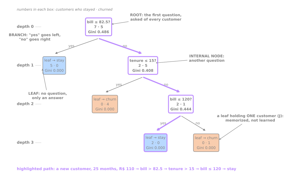
- The root is the first question, asked of every example. Each internal node asks another question, only of the examples that reached it.
- Every question has the form feature ≤ threshold. The left branch is "yes"; the right one, "no".
- A leaf asks nothing: it holds an answer (the majority class of the training examples that fell into it) and the counts behind it.
- The depth of a node is the number of questions between it and the root; the depth of the tree is that of its deepest node.
- Predicting is following a path: the highlighted customer has a R$ 110 bill (not ≤ 82.5, go right), 25 months as a client (not ≤ 15, go right) and a bill ≤ 120 (go left): "stay".
Look at the bottom-right leaf: it holds a single customer. Keep that picture in mind; it comes back in section 4.
2. Impurity: how mixed is a node?
A node is a group of examples. Let \(p_c\) be the share of class \(c\) in it. Two standard measures of how mixed it is:
Gini impurity (CART's default) — the probability that two examples drawn at random from the node, with replacement, belong to different classes:
Entropy (Quinlan's ID3 and C4.5) — the average number of bits needed to encode the class of an example drawn from the node:
Both are 0 for a pure node (one class only) and maximal for an even mix: with two classes, \(G = 0.5\) and \(H = 1\) at 50/50. For the root of our table, 7 stayed and 5 churned:
def gini(y):
    p = np.bincount(y, minlength=2) / len(y)
    return 1 - np.sum(p ** 2)

def entropy(y):
    p = np.bincount(y, minlength=2) / len(y)
    p = p[p > 0]
    return -np.sum(p * np.log2(p))

y_c = customers['churn'].to_numpy()
print(f"root: Gini {gini(y_c):.3f} · entropy {entropy(y_c):.3f}")
3. The best question: every split, scored
Stage 2. A question feature ≤ t splits a node of \(n\) examples into a left child with \(n_L\) and a right child with \(n_R\). The split is scored by the weighted impurity of the children, and its gain by how much that is below the parent's:
With entropy as \(I\), \(\Delta\) is called the information gain. The weights matter: a pure child of one example should not count as much as a pure child of six.
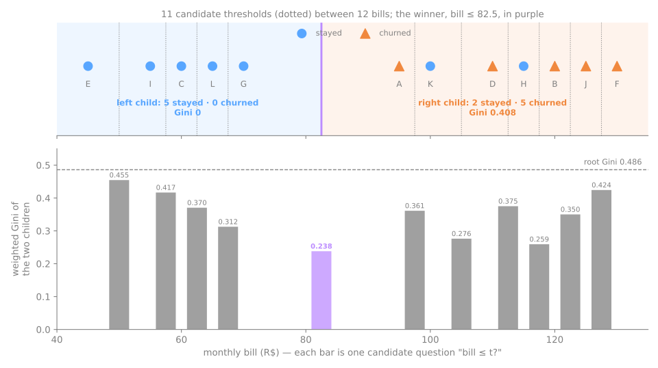
Which thresholds are worth trying? Between two consecutive distinct values of the feature, every threshold produces the same split, so only one per gap is needed; CART uses the midpoint. The 12 bills have 12 distinct values, hence 11 candidates:
def candidate_splits(feature):
    x = customers[feature].to_numpy()
    values = np.unique(x)                               # sorted distinct values
    rows = []
    for t in (values[:-1] + values[1:]) / 2:            # midpoints between neighbors
        left, right = y_c[x <= t], y_c[x > t]
        weighted = (len(left) * gini(left) + len(right) * gini(right)) / len(y_c)
        rows.append({'threshold': t,
                     'left (stay/churn)': f"{(left == 0).sum()}/{(left == 1).sum()}",
                     'right (stay/churn)': f"{(right == 0).sum()}/{(right == 1).sum()}",
                     'Gini left': gini(left), 'Gini right': gini(right),
                     'weighted Gini': weighted, 'decrease': gini(y_c) - weighted})
    return pd.DataFrame(rows)

table = candidate_splits('bill')
print(table.round(3).to_string(index=False))
best_tenure = candidate_splits('tenure').sort_values('weighted Gini').iloc[0]
print(f"best split on tenure: tenure <= {best_tenure['threshold']:g}, "
      f"weighted Gini {best_tenure['weighted Gini']:.3f}")
 threshold left (stay/churn) right (stay/churn)  Gini left  Gini right  weighted Gini  decrease
      50.0               1/0                6/5      0.000       0.496          0.455     0.032
      57.5               2/0                5/5      0.000       0.500          0.417     0.069
      62.5               3/0                4/5      0.000       0.494          0.370     0.116
      67.5               4/0                3/5      0.000       0.469          0.312     0.174
      82.5               5/0                2/5      0.000       0.408          0.238     0.248
      97.5               5/1                2/4      0.278       0.444          0.361     0.125
     105.0               6/1                1/4      0.245       0.320          0.276     0.210
     112.5               6/2                1/3      0.375       0.375          0.375     0.111
     117.5               7/2                0/3      0.346       0.000          0.259     0.227
     122.5               7/3                0/2      0.420       0.000          0.350     0.136
     127.5               7/4                0/1      0.463       0.000          0.424     0.062
best split on tenure: tenure <= 4, weighted Gini 0.350
Check the winning row with a calculator. bill ≤ 82.5 (the midpoint between R$ 70 and R$ 95) sends the 5 customers with the lowest bills left, all of whom stayed: Gini 0. The right child has 2 stayers and 5 churners:
No other threshold on bill comes close, and the best question on tenure (tenure ≤ 4, weighted Gini 0.350) is worse too. Notice that the decrease is not monotone along the table: bill ≤ 97.5 (0.125) is much worse than its neighbors, because it moves one churner into the left child and spoils its purity. The only way to find the best split is to score all of them.
The figure shows the whole search at once: the 12 customers in bill order, the 11 candidate thresholds between them and the score of each (figure script):
scikit-learn agrees
A tree limited to one split is called a stump. DecisionTreeClassifier(max_depth=1) must find exactly the split above:
from sklearn.tree import DecisionTreeClassifier, export_text

X_c = customers[['tenure', 'bill']]
stump = DecisionTreeClassifier(max_depth=1, random_state=0).fit(X_c, y_c)
t = stump.tree_
print("feature:", X_c.columns[t.feature[0]], "· threshold:", t.threshold[0])
print("node impurities (root, left, right):", t.impurity.round(3))
print(export_text(stump, feature_names=list(X_c.columns), show_weights=True))
stump_H = DecisionTreeClassifier(max_depth=1, criterion='entropy', random_state=0).fit(X_c, y_c)
print("with entropy:", X_c.columns[stump_H.tree_.feature[0]], "<=", stump_H.tree_.threshold[0],
      "· node entropies", stump_H.tree_.impurity.round(3))
feature: bill · threshold: 82.5
node impurities (root, left, right): [0.486 0.    0.408]
|--- bill <= 82.50
|   |--- weights: [5.00, 0.00] class: 0
|--- bill >  82.50
|   |--- weights: [2.00, 5.00] class: 1

with entropy: bill <= 82.5 · node entropies [0.98  0.    0.863]
Same feature, same threshold, same three Gini values (0.486, 0, 0.408). The fitted tree lives in tree_: parallel arrays indexed by node number, with feature, threshold, impurity, n_node_samples and value for each node. export_text prints it as indented rules, and show_weights=True adds the class counts in each leaf (stay, churn). With criterion='entropy' the stump picks the same split, with information gain \(0.980 - \tfrac{7}{12}\cdot 0.863 = 0.476\). This is the usual outcome: Gini and entropy disagree on only a small fraction of splits in practice (Raileanu & Stoffel, 2004), and Gini is slightly cheaper to compute because it needs no logarithm.
4. Growing the tree
Greedy and recursive
Stage 3. CART grows the whole tree by repeating the stump search inside each child:
GROW(node):
    if a stopping rule holds (node is pure, max_depth reached, too few samples): make a leaf
    for each feature j, for each midpoint t between consecutive values of j:
        score the split x_j <= t by the impurity decrease Δ
    apply the best split; GROW(left child); GROW(right child)
Two words describe it. Recursive: each child is a smaller version of the same problem. Greedy: each split is the best one now, with no lookahead; a split that looks poor alone but would enable an excellent split below it is never chosen. Finding the tree that is globally best is NP-complete (Hyafil & Rivest, 1976), so every practical algorithm is greedy. It is also fast: with the values of each feature sorted once, scoring all thresholds of a node costs one pass over its rows, so growing a tree costs roughly \(O(p\, n \log n)\) for \(n\) rows and \(p\) features.
On the churn table, the left child (bill ≤ 82.5) is pure and becomes a leaf. The right child (2 stay, 5 churn) is split again:
tree2 = DecisionTreeClassifier(max_depth=2, random_state=0).fit(X_c, y_c)
print(export_text(tree2, feature_names=list(X_c.columns), show_weights=True))

new = pd.DataFrame({'tenure': [6, 4, 25], 'bill': [70, 115, 110]}, index=['M', 'N', 'O'])
print(pd.DataFrame(tree2.predict_proba(new), index=new.index, columns=['P(stay)', 'P(churn)']).round(3)
      .assign(prediction=tree2.predict(new), leaf=tree2.apply(new)))
|--- bill <= 82.50
|   |--- weights: [5.00, 0.00] class: 0
|--- bill >  82.50
|   |--- tenure <= 15.00
|   |   |--- weights: [0.00, 4.00] class: 1
|   |--- tenure >  15.00
|   |   |--- weights: [2.00, 1.00] class: 0

   P(stay)  P(churn)  prediction  leaf
M    1.000     0.000           0     1
N    0.000     1.000           1     3
O    0.667     0.333           0     4
Inside the high-bill group, the best question is tenure ≤ 15: the 4 recent customers with high bills all churned. The tree and the partition of the plane it defines (figure script):
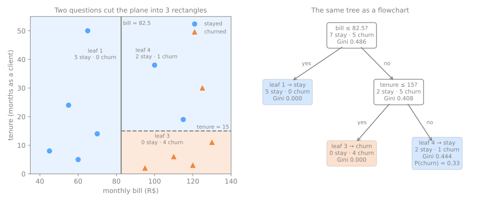
Every split is a vertical or horizontal line, and it only cuts the region of its own node: the line tenure = 15 stops at bill = 82.5. So a tree always partitions the feature space into axis-aligned rectangles (boxes, in more dimensions), one per leaf. The model is also a statement about interactions: tenure matters, but only for customers with high bills. A linear model would need an explicit product feature to say that; a tree says it by nesting one question inside another.
Leaves hold proportions
Look at the three new customers. M (bill 70) lands in leaf 1, where all 5 training customers stayed: P(churn) = 0. N (4 months, R$ 115) lands in leaf 3, where all 4 churned. O (25 months, R$ 110) lands in leaf 4, which holds 2 stayers and 1 churner: predict_proba returns the class proportions of the training examples in that leaf, \((2/3, 1/3)\), and predict returns the majority, "stay". apply tells you the leaf number (the node numbers used in the figure above). Every example in a leaf gets the same probability, so a tree with 3 leaves can output only 3 distinct probabilities; the ROC curve of such a model (the ROC and imbalanced data lesson) has only a few corners.
Grown to purity
Leaf 4 is still mixed. With no stopping rule, CART keeps splitting until every leaf is pure:
full = DecisionTreeClassifier(random_state=0).fit(X_c, y_c)
print(export_text(full, feature_names=list(X_c.columns), show_weights=True))
print(f"leaves: {full.get_n_leaves()} · depth: {full.get_depth()} · training accuracy: {full.score(X_c, y_c):.3f}")
|--- bill <= 82.50
|   |--- weights: [5.00, 0.00] class: 0
|--- bill >  82.50
|   |--- tenure <= 15.00
|   |   |--- weights: [0.00, 4.00] class: 1
|   |--- tenure >  15.00
|   |   |--- bill <= 120.00
|   |   |   |--- weights: [2.00, 0.00] class: 0
|   |   |--- bill >  120.00
|   |   |   |--- weights: [0.00, 1.00] class: 1

leaves: 4 · depth: 3 · training accuracy: 1.000
The third question, bill ≤ 120, exists to isolate a single customer: J, 30 months as a client, who churned with a bill of R$ 125. Is "long-time customers above R$ 120 churn" a pattern or an accident of one row? With one example there is no way to tell, and the tree does not ask; it reaches 100% training accuracy because it is allowed to. Keep this picture in mind: it is the whole overfitting story of this lesson, in miniature.
The figure gathers the four stages, from a single node to the pure tree, with the number of leaves and the training accuracy of each (figure script):
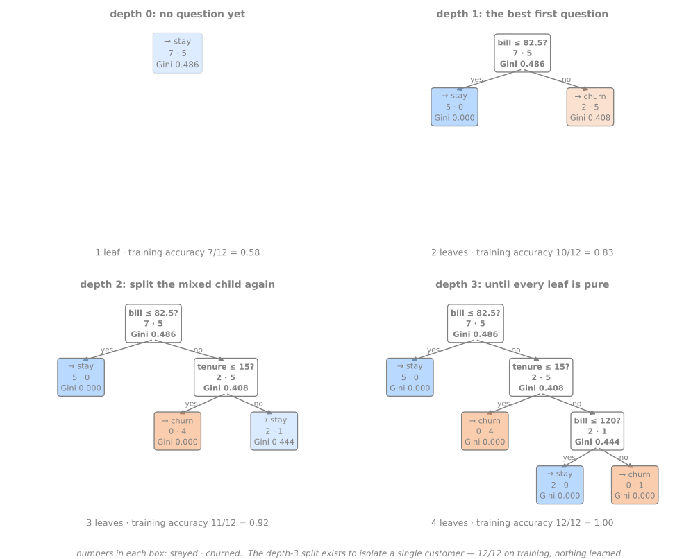
Training accuracy rises at every level: 0.58, 0.83, 0.92 and finally 1.00. The first two splits separate groups of 5 and 4 customers; the third exists because of one customer. Perfect training accuracy, for a tree without limits, is not an achievement: it is what the algorithm always does.
The simulator grows a tree one level at a time on 120 points. Raise the depth and watch the regions shatter into boxes around single points, while the training impurity keeps falling:
5. Overfitting and pre-pruning
A fully grown tree memorizes
Stage 4. The 12-customer table suggested it; a real dataset measures it. Spambase (Hopkins et al., 1999) has 4,601 e-mails described by 57 numbers: frequencies of words (word_freq_free, word_freq_hp), of characters (char_freq_$, char_freq_!) and runs of capital letters. The task is to flag spam. The development/test split and the cv object below are reused in the rest of the lesson:
from sklearn.datasets import fetch_openml
from sklearn.model_selection import StratifiedKFold, cross_validate, train_test_split
from urllib.parse import unquote

spam = fetch_openml(data_id=44, as_frame=True)          # Spambase: 4,601 e-mails, 57 features
X, y = spam.data, spam.target.astype(int)               # 1 = spam
X.columns = [unquote(c) for c in X.columns]             # 'char_freq_%24' -> 'char_freq_$'
repeated = X.duplicated()
print(f"{repeated.sum()} rows repeat an earlier row exactly: dropped")
X, y = X[~repeated], y[~repeated]
X_dev, X_test, y_dev, y_test = train_test_split(X, y, test_size=0.25, stratify=y, random_state=0)
print(X_dev.shape, X_test.shape, f"spam share {y_dev.mean():.3f}")

cv = StratifiedKFold(n_splits=5, shuffle=True, random_state=0)
res = cross_validate(DecisionTreeClassifier(random_state=0), X_dev, y_dev, cv=cv,
                     return_train_score=True, return_estimator=True)
print(f"training folds {res['train_score'].mean():.3f} · validation folds "
      f"{res['test_score'].mean():.3f} ± {res['test_score'].std():.3f}")
print("leaves per fold:", [int(m.get_n_leaves()) for m in res['estimator']],
      "· depth per fold:", [int(m.get_depth()) for m in res['estimator']])
394 rows repeat an earlier row exactly: dropped
(3155, 57) (1052, 57) spam share 0.399
training folds 1.000 · validation folds 0.906 ± 0.008
leaves per fold: [171, 187, 181, 188, 179] · depth per fold: [32, 28, 31, 30, 27]
First, 394 e-mails appear twice with identical features. Left in, a copy in a validation fold would be "predicted" by its twin in the training folds, the duplicate-row leak of the validation lesson, and a model that memorizes, like a fully grown tree, would profit most from it. We drop them.
Then the measurement: the fully grown tree scores 1.000 on the training folds and 0.906 on the validation folds. To get there it needs about 180 leaves and a depth near 30 for some 2,500 e-mails: many leaves hold one or two training e-mails, exactly like the leaf that isolated customer J above. Trees are low-bias, high-variance learners: nothing in the algorithm stops the recursion before every leaf is pure, and a pure leaf is a memorized example. Two families of remedies exist.
Pre-pruning: stop early
Stopping rules end the recursion before the leaves are pure. The main knobs of DecisionTreeClassifier:
max_depth— the longest path from root to leaf;min_samples_leaf— every leaf must keep at least this many training examples (a split that would create a smaller child is not allowed);max_leaf_nodes— grow best-first and stop at this many leaves;min_samples_split,min_impurity_decrease— do not split small nodes, or splits that gain too little.
settings = [{}, {'max_depth': 3}, {'max_depth': 10},
            {'min_samples_leaf': 5}, {'min_samples_leaf': 50},
            {'max_leaf_nodes': 8}, {'max_leaf_nodes': 40}]
rows = []
for s in settings:
    r = cross_validate(DecisionTreeClassifier(random_state=0, **s), X_dev, y_dev, cv=cv,
                       return_train_score=True, return_estimator=True)
    rows.append({'setting': str(s) if s else 'none (fully grown)',
                 'train': r['train_score'].mean(), 'validation': r['test_score'].mean(),
                 'std': r['test_score'].std(),
                 'leaves': np.mean([m.get_n_leaves() for m in r['estimator']])})
print(pd.DataFrame(rows).round(3).to_string(index=False))
                 setting  train  validation   std  leaves
      none (fully grown)  1.000       0.906 0.008   181.2
        {'max_depth': 3}  0.890       0.880 0.012     8.0
       {'max_depth': 10}  0.967       0.915 0.009    86.4
 {'min_samples_leaf': 5}  0.957       0.900 0.006   111.8
{'min_samples_leaf': 50}  0.902       0.892 0.012    30.4
   {'max_leaf_nodes': 8}  0.899       0.891 0.007     8.0
  {'max_leaf_nodes': 40}  0.950       0.906 0.004    40.0
Every knob moves the tree along the same bias–variance axis. Too tight (max_depth=3, 8 leaves) and both training and validation accuracy are low, 0.890 and 0.880: underfitting, visible because the two numbers sit together. Too loose (no limit) and training accuracy reaches 1.000 while validation stays at 0.906. In between, max_depth=10 reaches 0.915 with 86 leaves. The more striking line is max_leaf_nodes=40: the same validation accuracy as the fully grown tree (0.906) with 40 leaves instead of 181. The extra 140 leaves were spent memorizing.
6. Reading a tree: a path is a rule
Stage 5. The main reason to use a single tree instead of an ensemble is that a person can read it. A depth-2 tree on Spambase:
small = DecisionTreeClassifier(max_depth=2, random_state=0).fit(X_dev, y_dev)
print(export_text(small, feature_names=list(X.columns), show_weights=True))
print(f"test accuracy of this 4-leaf tree: {small.score(X_test, y_test):.3f}")
|--- char_freq_$ <= 0.05
|   |--- word_freq_remove <= 0.06
|   |   |--- weights: [1770.00, 356.00] class: 0
|   |--- word_freq_remove >  0.06
|   |   |--- weights: [19.00, 211.00] class: 1
|--- char_freq_$ >  0.05
|   |--- word_freq_hp <= 0.38
|   |   |--- weights: [50.00, 687.00] class: 1
|   |--- word_freq_hp >  0.38
|   |   |--- weights: [57.00, 5.00] class: 0

test accuracy of this 4-leaf tree: 0.863
Each root-to-leaf path is an if–then rule, and the weights say how much training data supports it (not spam, spam):
- if
$is rare (≤ 0.05% of characters) andremoveis rare: not spam — 1,770 legitimate e-mails against 356 spams; - if
$is rare butremoveappears (as in "click here to be removed from the list"): spam, 211 against 19; - if
$is frequent andhpis rare: spam, 687 against 50; - if
$is frequent buthpappears: not spam, 57 against 5. The data were collected at Hewlett-Packard, and a message mentioninghpwas most likely internal mail.
Four rules, 0.863 on the test set: 6 points below the fully grown tree (0.923 on the test set, as section 12 will measure), with 4 leaves instead of 221, and a model anyone can check. The last rule also shows why reading matters: it is true in this dataset and useless anywhere else, and you only find that out by looking. plot_tree draws the same tree as a diagram (you will use it in the lab).
7. Summary: a tree in five lines
- A tree asks questions feature ≤ threshold, one at a time, from the root to a leaf; predicting is following a path.
- A good question leaves the children purer. Impurity (Gini or entropy) measures the mixing; a split is scored by the weighted impurity of its children.
- The best split is found by brute force: every feature, every midpoint between neighboring values.
- Growth is greedy and recursive: the best split now, repeated inside each child, until a stopping rule.
- Without a stopping rule, the tree memorizes: pure leaves, perfect training.
max_depth,min_samples_leafandmax_leaf_nodeshold it back; cross-validation chooses how much.
| symptom | what is happening | what to do |
|---|---|---|
| training accuracy 1.000, validation well below | the tree memorized the training set | limit the depth or the leaf size |
| training and validation both low and close | the tree is too shallow | let it grow one more level |
| hundreds of leaves for a few thousand rows | leaves with one or two examples | min_samples_leaf or max_leaf_nodes |
| a small tree scores almost as well as the big one | the extra leaves only memorized | keep the small one: it can be read |
Fundamental lab — a key for penguins
The problem. Field guides identify species with a dichotomous key: a list of yes/no questions ("bill longer than 43 mm? go to 5; otherwise go to 7") that ends at a species name. A dichotomous key is a decision tree written by hand. The Palmer penguins dataset (Gorman et al., 2014) has 344 penguins of three species, Adelie, Chinstrap and Gentoo, measured on three islands of the Palmer Archipelago, Antarctica: bill (culmen) length and depth, flipper length, body mass, sex and island. The field team wants a key small enough to print on a card, and wants to know what that readability costs in accuracy compared with models nobody can read.
The workflow is the one from the validation lesson: lock away a test set, use one cv object for everything, and touch the test set exactly once, at step 8. This part prepares the data, builds and reads a depth-2 key, and lets the tree grow all the way; tuning, comparing with other models and testing are left to the advanced lab.
How to do this lab in class (about 30 min, in pairs)
- Open the lab notebook on Colab (in Portuguese). There is nothing to download or install: Colab runs in the browser. To keep your answers, save a copy to your Drive (File → Save a copy in Drive) before editing. Run the cells in order, in a single session.
- This lab is steps 1 to 5 of the notebook. The advanced lab continues in the same notebook, from step 6.
- Every step starts with a Predict: answer it with your partner before running the cell. Getting the prediction wrong is what makes the result memorable.
- After running, compare with the output and the reading on this page. Every output here is exactly what the code prints.
- The Simulations ask you to write a small Python experiment: change one input and watch what happens to the output. No hand calculations. The solution is collapsed right below: try before opening it.
- Suggested pace: steps 1 to 3 in 8 min; step 4 and the first simulation in 12 min; step 5 and the second simulation in 10 min.
Step 1 — load and look
Predict. There are three penguin species. Do you expect them in similar proportions? What accuracy would a model that always answers the most common species get?
import numpy as np
import pandas as pd
from sklearn.datasets import fetch_openml

peng = fetch_openml(data_id=42585, as_frame=True).frame      # Palmer penguins
print(peng.shape)
print(peng['species'].value_counts().to_dict())
print(peng.isna().sum().to_dict())
print(peng['sex'].value_counts(dropna=False).to_dict())
(344, 7)
{'Adelie': 152, 'Gentoo': 124, 'Chinstrap': 68}
{'species': 0, 'island': 0, 'culmen_length_mm': 2, 'culmen_depth_mm': 2, 'flipper_length_mm': 2, 'body_mass_g': 2, 'sex': 10}
{'MALE': 168, 'FEMALE': 165, nan: 10, '_': 1}
344 penguins: 152 Adelie, 124 Gentoo and only 68 Chinstrap, so accuracy must be read against a majority baseline of 44%. Two birds have no measurement at all. The sex column has 10 missing values and one entry, '_', that is neither sex: a data-entry error, to be treated as missing.
Step 2 — clean and encode
Predict. A tree accepts NaN and needs no scaling. Of the three usual cleaning steps — impute, scale, encode categories —, which one is still needed here?
num = ['culmen_length_mm', 'culmen_depth_mm', 'flipper_length_mm', 'body_mass_g']
peng = peng.dropna(subset=num)                    # the 2 birds with no measurement at all
X = peng[num].copy()
X['is_male'] = peng['sex'].astype(object).map({'MALE': 1.0, 'FEMALE': 0.0})   # '_' and unknown -> NaN
X = X.join(pd.get_dummies(peng['island'], prefix='island', dtype=float))      # one-hot
y = peng['species'].astype(str)
print(X.shape)
print("missing:", X.isna().sum()[X.isna().sum() > 0].to_dict())
print(X.head(3).to_string())
(342, 8)
missing: {'is_male': 9}
   culmen_length_mm  culmen_depth_mm  flipper_length_mm  body_mass_g  is_male  island_Biscoe  island_Dream  island_Torgersen
0              39.1             18.7              181.0       3750.0      1.0            0.0           0.0               1.0
1              39.5             17.4              186.0       3800.0      0.0            0.0           0.0               1.0
2              40.3             18.0              195.0       3250.0      0.0            0.0           0.0               1.0
342 penguins and 8 numeric columns. island is categorical, so it becomes three 0/1 columns (one-hot). sex becomes is_male, with NaN for the 9 remaining penguins whose sex is unknown. We keep those NaN: the tree accepts them as they are, and the rivals of step 7 will get an imputer inside their pipelines. Nothing is scaled; the tree does not need it.
Step 3 — lock the test set away, and a baseline
Predict. With 86 test penguins, how many accuracy points is a single error worth? Does that change how much you should trust the third decimal place?
from sklearn.dummy import DummyClassifier
from sklearn.model_selection import StratifiedKFold, cross_validate, train_test_split

X_train, X_test, y_train, y_test = train_test_split(X, y, test_size=0.25, stratify=y, random_state=42)
print(X_train.shape, X_test.shape)

cv = StratifiedKFold(n_splits=5, shuffle=True, random_state=42)


def cv_report(model):
    r = cross_validate(model, X_train, y_train, cv=cv, return_train_score=True)
    return (f"train {r['train_score'].mean():.3f} · validation "
            f"{r['test_score'].mean():.3f} ± {r['test_score'].std():.3f}")


print("dummy:", cv_report(DummyClassifier(strategy='most_frequent')))
256 penguins for development and 86 locked away until step 8, with the species proportions preserved by stratify=y. With 86 test birds, one mistake costs 1.2 points of accuracy. Always answering "Adelie" scores 0.441. cv_report prints the mean training and validation accuracy over the same five folds, which every later step reuses.
Step 4 — a depth-2 tree, read as rules
Predict. Can a single question (depth 1) separate three species? And with two questions in sequence, which measurement do you think the root will use?
import matplotlib.pyplot as plt
from sklearn.tree import DecisionTreeClassifier, export_text, plot_tree

print("depth 1:", cv_report(DecisionTreeClassifier(max_depth=1, random_state=0)))
print("depth 2:", cv_report(DecisionTreeClassifier(max_depth=2, random_state=0)))

tree2 = DecisionTreeClassifier(max_depth=2, random_state=0).fit(X_train, y_train)
print(tree2.classes_)
print(export_text(tree2, feature_names=list(X.columns), show_weights=True))

plot_tree(tree2, feature_names=list(X.columns), class_names=list(tree2.classes_),
          filled=True, rounded=True, fontsize=8)
plt.show()
depth 1: train 0.785 · validation 0.770 ± 0.034
depth 2: train 0.960 · validation 0.938 ± 0.040
['Adelie' 'Chinstrap' 'Gentoo']
|--- flipper_length_mm <= 206.50
|   |--- culmen_length_mm <= 43.35
|   |   |--- weights: [107.00, 4.00, 0.00] class: Adelie
|   |--- culmen_length_mm >  43.35
|   |   |--- weights: [4.00, 42.00, 1.00] class: Chinstrap
|--- flipper_length_mm >  206.50
|   |--- culmen_depth_mm <= 17.55
|   |   |--- weights: [0.00, 0.00, 91.00] class: Gentoo
|   |--- culmen_depth_mm >  17.55
|   |   |--- weights: [2.00, 5.00, 0.00] class: Chinstrap
How to read it:
- One question is not enough. A stump can have only two leaves, so it can name only two of the three species: 0.770.
- Two levels already make a usable key, 0.938 ± 0.040, with four rules. The weights are counts of (Adelie, Chinstrap, Gentoo) in each leaf. Long flippers (> 206.5 mm) and a shallow bill (≤ 17.55 mm) is Gentoo: 91 of 91. Short flippers and a short bill (≤ 43.35 mm) is Adelie: 107 of 111. Short flippers and a long bill is Chinstrap: 42 of 47.
- The mistakes are where the species overlap. Adelie and Chinstrap have similar flippers and differ mainly in bill length: 8 of the 9 misplaced birds in the two left leaves are Adelies and Chinstraps on the wrong side of the 43.35 mm threshold. The fourth leaf (long flippers, deep bill) holds only 7 birds, a mix of Adelie and Chinstrap.
plot_tree draws the same tree; each box shows the question, the Gini of the node, the number of samples, the class counts (value) and the majority class, colored by class and purity.
Simulation: the root, chosen by you. Section 3 scored by hand every split of a 12-customer table. Do the same with the penguins: for each of the four measurements, try every midpoint between neighboring values in X_train, score each split by its weighted Gini (now with three classes) and keep the best. Is the winning question the root that the tree of step 4 chose? By how much does it win?
Solution
def gini_counts(labels):
    p = labels.value_counts(normalize=True).to_numpy()     # species fractions in the node
    return 1 - np.sum(p ** 2)

print(f"root Gini: {gini_counts(y_train):.3f}")
for col in ['culmen_length_mm', 'culmen_depth_mm', 'flipper_length_mm', 'body_mass_g']:
    x = X_train[col].to_numpy()
    values = np.unique(x)
    best = (np.inf, None)
    for t in (values[:-1] + values[1:]) / 2:               # midpoints between neighbors
        left, right = y_train[x <= t], y_train[x > t]
        w = (len(left) * gini_counts(left) + len(right) * gini_counts(right)) / len(y_train)
        best = min(best, (w, t))
    print(f"{col:18s} {len(values) - 1:3d} thresholds · best <= {best[1]:7.2f} · weighted Gini {best[0]:.3f}")
root Gini: 0.636
culmen_length_mm   144 thresholds · best <=   42.30 · weighted Gini 0.324
culmen_depth_mm     75 thresholds · best <=   16.40 · weighted Gini 0.331
flipper_length_mm   51 thresholds · best <=  206.50 · weighted Gini 0.312
body_mass_g         89 thresholds · best <= 4525.00 · weighted Gini 0.400
That is 359 candidate questions (144 + 75 + 51 + 89), and the winner is exactly the root of step 4, flipper_length_mm <= 206.50, with a weighted Gini of 0.312. But the win is narrow: the best split on bill length scores 0.324 and the best on bill depth 0.331. Three almost equally good questions compete for the root, so a small change in the data can swap the winner — keep that in mind for step 10. Body mass (0.400) separates much worse: weighing the bird is not enough. And with three classes the root Gini is 0.636, above the 0.5 maximum it reaches with two: with \(K\) balanced classes the maximum is \(1 - 1/K\).
Step 5 — grow it all the way
Predict. With no limit at all, does the tree reach 100% accuracy on training? And on validation: will it get worse than the depth-2 tree, as on Spambase, or better?
full = DecisionTreeClassifier(random_state=0)
print("fully grown:", cv_report(full))
full.fit(X_train, y_train)
print(f"depth {full.get_depth()} · {full.get_n_leaves()} leaves for {len(X_train)} penguins")
The fully grown tree fits the training folds perfectly (1.000) and scores 0.969 ± 0.016 in validation, better than depth 2. Unlike Spambase, penguins are easy and clean: the full tree needs only 13 leaves, so there is little to memorize. But 13 leaves is not a card-sized key.
Simulation: a tree memorizes even random labels. Shuffle the species of y_train — every penguin gets the species of another one, drawn at random — and repeat the cross-validation of the fully grown tree. What happens to the training accuracy? And to the validation accuracy? Compare also the number of leaves with that of the tree on the real labels.
Solution
shuffled = y_train.sample(frac=1, random_state=0).to_numpy()      # the species, shuffled
r = cross_validate(DecisionTreeClassifier(random_state=0), X_train, shuffled, cv=cv,
                   return_train_score=True, return_estimator=True)
print(f"random labels: train {r['train_score'].mean():.3f} · validation {r['test_score'].mean():.3f}"
      f" · {np.mean([m.get_n_leaves() for m in r['estimator']]):.0f} leaves for ~205 penguins")
print(f"real labels:   {cv_report(full)}")
random labels: train 1.000 · validation 0.355 · 84 leaves for ~205 penguins
real labels:   train 1.000 · validation 0.969 ± 0.016
With random labels there is nothing to learn and yet the tree reaches 1.000 on the training folds: it grows until every leaf is pure, whatever it takes — 84 leaves for about 205 penguins per fold, against the 13 of the step-5 tree on all 256. Validation collapses to 0.355, below even the 0.441 baseline: the memorized rules are worthless on new penguins. The lesson: the training accuracy of a fully grown tree says nothing, because it is 1.000 with signal or without. Only validation tells the two cases apart; the number of leaves is a good alarm.
To close the fundamental part. In one sentence each: (1) what makes one question better than another? (2) Why does a fully grown tree reach 100% training accuracy, even with random labels? (3) How would you read aloud a path from the root to a leaf of the step-4 key?
Your turn (fundamental)
At home:
- Entropy. Redo step 4 with
criterion='entropy'. Does the depth-2 tree choose the same questions? And the same thresholds? - Information gain by hand. On the 12-customer table, compute by hand the entropy of the two children of
bill ≤ 82.5and the information gain of the split. Check it against the 0.476 of section 3. - Minimum leaves instead of depth. Redo step 5 with
min_samples_leaf=5and withmin_samples_leaf=10. How many leaves does the tree have, and what happens to training and validation accuracy?
Advanced approach
The fundamental part grew a tree and stopped it from memorizing. This part shows where trees shine and where they fail: why the split criterion cannot be the error rate, how a tree does regression (and why it cannot extrapolate), how to prune after growing, why a tree changes so much with the data, and what it does — and does not — spare you compared with other models. The code blocks continue those of sections 1 to 6.
This part follows one path in four stages, drawn below: 1. measure the split; 2. prune after growing; 3. face the instability; 4. strengths and limits. Each stage links to its section, and in the slides a strip at the bottom shows which stage you are in.
- Measure the splitimpurity, not errors; variance for regression
- Prune after growingcost-complexity pruning and the choice of α
- Face the instabilitya small change in the data, a different tree
- Strengths and limitsscaling, staircases,
NaN, importance
Advanced approach slides
Click the slides and use the ← → arrows to navigate; F opens full screen and Esc shows every slide. Open the slides in a new tab
8. Why not simply count errors?
Stage 1. The most obvious measure of how mixed a node is would be its misclassification rate: the share of examples that are not of the majority class, \(1 - \max_c p_c\). It is what we finally care about, so why not split on it? The figure shows the three measures side by side, and a split that exposes the problem (figure script):
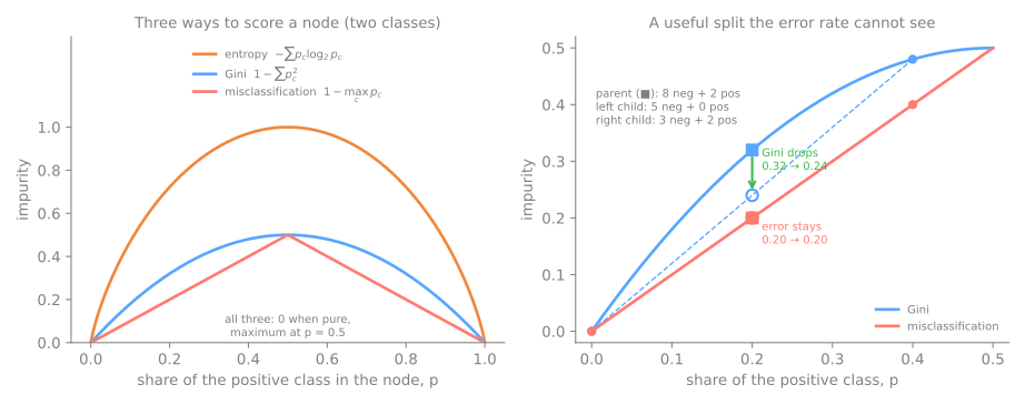
The parent has 8 negatives and 2 positives, so it predicts "negative" and makes 2 errors in 10. The split sends 5 negatives to a pure left child and leaves 3 negatives and 2 positives on the right. Both children still predict "negative", and the right one still makes exactly the same 2 errors: the misclassification rate stays at \(0.20\), and the split looks worthless. Yet it is a good first step: one child is pure and finished, and the positives are now concentrated in a node of 5 where the next question can isolate them. Gini sees this progress, falling from \(0.32\) to \(\tfrac{5}{10}\cdot 0 + \tfrac{5}{10}\cdot 0.48 = 0.24\).
The right panel shows why geometrically. The weighted impurity of the children is a point on the chord between the two children's points, taken at the parent's \(p\). The misclassification rate is a straight line between 0 and 0.5, so the chord lies on the curve and the decrease is zero. Gini and entropy are strictly concave, so the chord lies below the curve and every split that changes the class proportions shows a positive decrease. Growing a tree is a sequence of steps whose value often appears only one level later; a criterion that rewards progress, not just finished decisions, is what makes the greedy search work.
9. Regression trees
Variance reduction, by hand
For a numeric target, the same algorithm works with a different impurity. A leaf predicts the mean of its training targets, so a natural impurity is the mean squared error around that mean, which is the variance of the target in the node:
A split is scored exactly as before, by the weighted impurity of the children. Eight apartments, area in m² and monthly rent in R$ thousand:
from sklearn.tree import DecisionTreeRegressor

flats = pd.DataFrame({'area': [30, 38, 45, 52, 60, 75, 90, 110],             # m²
                      'rent': [1.3, 1.5, 1.6, 2.0, 2.2, 3.1, 3.4, 3.8]})      # R$ thousand / month
area, rent = flats['area'].to_numpy(), flats['rent'].to_numpy()
mse = lambda v: np.mean((v - v.mean()) ** 2)                # impurity of a regression node
print(f"root: mean {rent.mean():.3f} · MSE {mse(rent):.4f}")

rows = []
for t in (area[:-1] + area[1:]) / 2:
    left, right = rent[area <= t], rent[area > t]
    weighted = (len(left) * mse(left) + len(right) * mse(right)) / len(rent)
    rows.append({'threshold': t, 'mean left': left.mean(), 'mean right': right.mean(),
                 'weighted MSE': weighted, 'decrease': mse(rent) - weighted})
print(pd.DataFrame(rows).round(4).to_string(index=False))

reg = DecisionTreeRegressor(max_depth=1).fit(flats[['area']], rent)
print(export_text(reg, feature_names=['area'], decimals=3))
root: mean 2.362 · MSE 0.7873
 threshold  mean left  mean right  weighted MSE  decrease
      34.0     1.3000      2.5143        0.6261    0.1613
      41.5     1.4000      2.6833        0.4785    0.3088
      48.5     1.4667      2.9000        0.3058    0.4815
      56.0     1.6000      3.1250        0.2059    0.5814
      67.5     1.7200      3.4333        0.0993    0.6880
      82.5     1.9500      3.6000        0.2769    0.5105
     100.0     2.1571      3.8000        0.4921    0.2952
|--- area <= 67.500
|   |--- value: [1.720]
|--- area >  67.500
|   |--- value: [3.433]
Before any split, the best constant prediction is the mean, R$ 2.362 thousand, with MSE 0.7873. The split area ≤ 67.5 predicts R$ 1.720 thousand for the five small apartments and R$ 3.433 thousand for the three large ones, and brings the weighted MSE down to 0.0993: one question removes \(0.688 / 0.787 = 87\%\) of the variance. DecisionTreeRegressor finds the same threshold and the same two leaf values.
A step function that cannot extrapolate
A regression tree with \(L\) leaves predicts at most \(L\) different values, so its prediction curve is a step function. The figure fits trees of depth 1 and 3 and a linear regression to 60 apartments between 30 and 120 m², where the true relation is a straight line plus noise, and scores them on fresh apartments inside and outside that range (figure script):
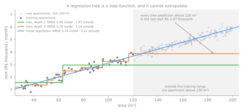
Inside the training range, the depth-3 staircase follows the line reasonably well (RMSE 0.29 against 0.24 for the linear model, which has the right shape by construction). Outside it, every apartment larger than 120 m² falls into the last leaf and gets the same prediction, R$ 3.87 thousand, however big it is: RMSE 1.14, five times the linear model's 0.22. A tree cannot extrapolate: it can only return averages of targets it has seen. For sales that grow over time, prices under inflation, or any target that must go beyond its training range, this matters, and it applies to the forests and boosted ensembles built from trees, too.
10. Post-pruning: grow, then cut back
Stage 2. Stopping rules have a weakness that comes from greediness: a split that gains little may enable a large gain below it, and an early stop never finds out. CART's answer (Breiman et al., 1984) is the reverse procedure: grow the full tree, then prune it back. Pruning uses the cost-complexity criterion, which charges a price \(\alpha\) per leaf:
where \(R(T)\) is the total impurity of the leaves of tree \(T\) (each leaf's impurity weighted by its share of the training rows) and \(|T|\) is the number of leaves. It is the tree version of regularization: \(\alpha = 0\) keeps the full tree, and larger \(\alpha\) makes leaves more expensive. For each internal node \(t\), collapsing its subtree \(T_t\) into a single leaf saves \(|T_t| - 1\) leaves and costs \(R(t) - R(T_t)\) in impurity, so it pays off once
Weakest-link pruning collapses the node with the smallest \(\alpha_{\text{eff}}\), recomputes, and repeats, producing a nested sequence of subtrees down to the root alone. On the full churn tree (4 leaves, all pure, so \(R(T) = 0\)), by hand:
- node
bill ≤ 120(3 customers: 2 stay, 1 churn; Gini 0.444): \(R(t) = \tfrac{3}{12}\cdot 0.444 = 0.111\), its subtree has 2 leaves, so \(\alpha_{\text{eff}} = 0.111 / 1 = 0.111\); - node
tenure ≤ 15(7 customers, Gini 0.408): \(R(t) = \tfrac{7}{12}\cdot 0.408 = 0.238\), 3 leaves: \(0.238 / 2 = 0.119\); - the root: \(0.486 / 3 = 0.162\).
The weakest link is bill ≤ 120, pruned at \(\alpha = 0.111\), which removes exactly the split that isolated customer J. Recomputing on the 3-leaf tree, tenure ≤ 15 now saves one leaf for \(0.238 - 0.111 = 0.127\), and the root goes last, at \(0.486 - 0.238 = 0.248\). scikit-learn computes the same sequence:
path_c = DecisionTreeClassifier(random_state=0).cost_complexity_pruning_path(X_c, y_c)
for a, imp in zip(path_c.ccp_alphas, path_c.impurities):
    leaves = DecisionTreeClassifier(random_state=0, ccp_alpha=a).fit(X_c, y_c).get_n_leaves()
    print(f"ccp_alpha {a:.3f} -> {leaves} leaves, total leaf impurity {imp:.3f}")
ccp_alpha 0.000 -> 4 leaves, total leaf impurity 0.000
ccp_alpha 0.111 -> 3 leaves, total leaf impurity 0.111
ccp_alpha 0.127 -> 2 leaves, total leaf impurity 0.238
ccp_alpha 0.248 -> 1 leaves, total leaf impurity 0.486
The figure shows the same sequence as trees: at every stage, the internal node with the smallest \(\alpha_{\text{eff}}\) (in purple) is the next one to become a leaf (figure script):
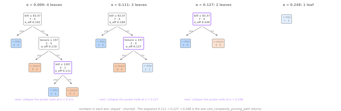
Which \(\alpha\) to use is a hyperparameter question, answered by cross-validation. On Spambase, the path of the full tree has over a hundred breakpoints; a log-spaced grid of 22 values covers it:
from sklearn.model_selection import GridSearchCV

path = DecisionTreeClassifier(random_state=0).cost_complexity_pruning_path(X_dev, y_dev)
print(f"{len(path.ccp_alphas)} breakpoints, from {path.ccp_alphas[1]:.5f} to {path.ccp_alphas[-1]:.4f}")

alphas = np.r_[0, np.geomspace(1e-4, 1e-2, 21)]
search = GridSearchCV(DecisionTreeClassifier(random_state=0), {'ccp_alpha': alphas}, cv=cv)
search.fit(X_dev, y_dev)
res = pd.DataFrame({'ccp_alpha': alphas,
                    'leaves': [DecisionTreeClassifier(random_state=0, ccp_alpha=a).fit(X_dev, y_dev).get_n_leaves()
                               for a in alphas],
                    'validation': search.cv_results_['mean_test_score'],
                    'std': search.cv_results_['std_test_score']})
print(res.iloc[::2].round(5).to_string(index=False))

b = search.best_index_
se = res.loc[b, 'std'] / np.sqrt(5)                     # standard error of the best mean
simplest = res[res['validation'] >= res.loc[b, 'validation'] - se]['leaves'].idxmin()
for name, i in [('best', b), ('1-SE rule', simplest)]:
    print(f"{name:9s}: ccp_alpha {res.loc[i, 'ccp_alpha']:.5f} · {res.loc[i, 'leaves']} leaves · "
          f"validation {res.loc[i, 'validation']:.3f}")
122 breakpoints, from 0.00008 to 0.1479
 ccp_alpha  leaves  validation     std
   0.00000     221     0.90650 0.00845
   0.00013     213     0.90650 0.00845
   0.00020     213     0.90681 0.00847
   0.00032     160     0.90745 0.00877
   0.00050     109     0.91537 0.00767
   0.00079      68     0.91442 0.00567
   0.00126      40     0.90777 0.00811
   0.00200      26     0.90365 0.00779
   0.00316      15     0.89540 0.00961
   0.00501       8     0.89128 0.00741
   0.00794       7     0.89287 0.00706
best     : ccp_alpha 0.00050 · 109 leaves · validation 0.915
1-SE rule: ccp_alpha 0.00100 · 57 leaves · validation 0.913
(The table prints every second row of the grid; the leaf counts are those of the tree pruned on all of X_dev.) Pruning from 221 to 109 leaves raises validation accuracy from 0.906 to 0.915; below about 40 leaves it starts to fall, to 0.891 at 8 leaves. The one-standard-error rule of the validation lesson, which comes from this very book (Breiman et al., 1984), takes the simplest tree whose score is within one standard error of the best: 57 leaves at 0.913, a quarter of the full tree, for a loss the folds cannot distinguish from zero. The figure shows both families of remedies side by side (figure script):
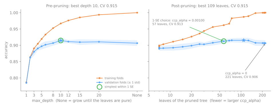
The two panels have the same shape as the C curve of logistic regression and the k curve of k-NN: training accuracy climbs with complexity, validation accuracy rises, flattens, and slowly falls. Pruning does not buy much accuracy here (0.906 to 0.915). Its larger gift is the size: a tree a quarter as large, just as accurate, and much easier to read.
11. Instability: a small change, a different tree
Stage 3. A tree is built from a cascade of choices, each made on the data that reached that node. Change a few rows and the root may pick another feature or another threshold; everything below it then changes too. To measure this, refit the fully grown tree on 50 bootstrap resamples of the development set (as many rows as the original, drawn with replacement, so each resample leaves out about a third of the rows and repeats others), and compare the 50 trees on the same test e-mails:
rng = np.random.default_rng(0)
roots, preds = [], []
for b in range(50):
    idx = rng.integers(0, len(X_dev), len(X_dev))            # a bootstrap resample
    m = DecisionTreeClassifier(random_state=0).fit(X_dev.iloc[idx], y_dev.iloc[idx])
    roots.append((X.columns[m.tree_.feature[0]], m.tree_.threshold[0], m.get_n_leaves()))
    preds.append(m.predict(X_test))
preds = np.array(preds)
roots = pd.DataFrame(roots, columns=['root feature', 'threshold', 'leaves'])
print(roots.groupby('root feature')['threshold'].agg(['count', 'min', 'max']).round(3))
print(f"leaves: from {roots['leaves'].min()} to {roots['leaves'].max()}")

acc = (preds == y_test.to_numpy()).mean(axis=1)
disagree = np.mean([np.mean(preds[i] != preds[j]) for i in range(50) for j in range(i + 1, 50)])
print(f"accuracy of each tree on the test rows: {acc.mean():.3f} (from {acc.min():.3f} to {acc.max():.3f})")
print(f"two trees disagree on {disagree:.1%} of the test e-mails")
print(f"majority vote of the 50 trees: {np.mean((preds.mean(axis=0) > 0.5) == y_test.to_numpy()):.3f}")
                  count    min    max
root feature
char_freq_!          19  0.067  0.150
char_freq_$          29  0.039  0.058
word_freq_free        1  0.015  0.015
word_freq_remove      1  0.010  0.010
leaves: from 136 to 186
accuracy of each tree on the test rows: 0.895 (from 0.873 to 0.919)
two trees disagree on 11.8% of the test e-mails
majority vote of the 50 trees: 0.950
The root question itself changes: char_freq_$ in 29 of the 50 trees, char_freq_! in 19, and two other words once each, with the threshold of each feature moving too. The trees have between 136 and 186 leaves. Their accuracies are similar, 0.895 on average; what differs is which e-mails they get wrong: two trees disagree on 11.8% of the test e-mails, about as often as either of them is wrong. That is what high variance means in practice. The same happens in two dimensions, where it can be seen (figure script):
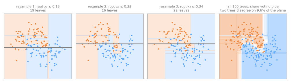
The last line of the output is a preview. Each tree is individually unreliable, but their errors are partly independent, so letting the 50 trees vote gives 0.950, better than the best single tree (0.919). Averaging many trees fitted on bootstrap resamples is called bagging; adding randomness in the features each split may consider turns it into the random forest, the subject of the next lesson. Instability is the defect of one tree and the raw material of the ensemble.
12. What trees do not need, and what they struggle with
No scaling needed
Stage 4. A split x ≤ t only uses the order of the values of one feature. Any strictly increasing transformation of a feature preserves that order, so the tree can find the same partition. Measured on Spambase:
from sklearn.preprocessing import StandardScaler

base = DecisionTreeClassifier(random_state=0).fit(X_dev, y_dev)
scaler = StandardScaler().fit(X_dev)
scaled = DecisionTreeClassifier(random_state=0).fit(scaler.transform(X_dev), y_dev)
logged = DecisionTreeClassifier(random_state=0).fit(np.log1p(X_dev), y_dev)

p = base.predict(X_test)
print(f"standardized: same prediction on {np.mean(scaled.predict(scaler.transform(X_test)) == p):.1%} of test rows")
print(f"log1p:        same prediction on {np.mean(logged.predict(np.log1p(X_test)) == p):.1%} of test rows, "
      f"{np.mean(logged.predict(np.log1p(X_dev)) == base.predict(X_dev)):.1%} of training rows")
print(f"test accuracy: raw {base.score(X_test, y_test):.3f} · standardized "
      f"{scaled.score(scaler.transform(X_test), y_test):.3f} · log1p {logged.score(np.log1p(X_test), y_test):.3f}")
standardized: same prediction on 100.0% of test rows
log1p:        same prediction on 99.3% of test rows, 100.0% of training rows
test accuracy: raw 0.923 · standardized 0.923 · log1p 0.922
Standardizing is a linear map, and it changes nothing: the same predictions on 100% of the test rows. The logarithm changes the order of nothing either, and the training predictions are identical; yet 0.7% of the test predictions differ. The reason is the midpoint. Between two neighboring training values \(a < b\), the raw tree puts its threshold at \((a+b)/2\); the log tree puts it at the midpoint of \(\log(1+a)\) and \(\log(1+b)\), which on the raw scale is \(\sqrt{(1+a)(1+b)} - 1\), a little below \((a+b)/2\). A new value that falls between those two thresholds goes left in one tree and right in the other. The partition of the training rows is identical; only the no-man's-land between them moves. So: no scaling is ever needed, and a monotone transformation changes a tree only at the margins, while it can change a linear model or k-NN completely. This is why trees are the usual choice for messy tabular data with skewed, heavy-tailed columns such as incomes or counts.
Interactions come for free
The churn tree used tenure only inside the high-bill branch: an interaction, "tenure matters when the bill is high". Logistic regression would need you to create the product tenure × bill or a similar feature by hand; a tree discovers such conditional effects by nesting questions. This is one reason trees and their ensembles do so well on tabular data where nobody knows in advance which combinations matter.
Diagonal boundaries become staircases
The flip side of splitting on one feature at a time: a boundary that depends on a combination of features, such as \(x_2 > x_1\), can only be approximated by many small axis-aligned steps (figure script):
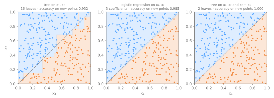
The tree needs 16 leaves for what logistic regression says with one line, and it is still worse on new points (0.932 against 0.985), because the steps are placed where the 300 training points happen to fall. Give the tree the feature \(x_2 - x_1\), and a single split solves the problem perfectly. Feature engineering that exposes the right combination helps a tree more than any hyperparameter.
Categorical features and missing values
Categorical features. In principle a tree can split a categorical feature directly: CART sends a subset of the categories to each side, and C4.5 makes one branch per category. scikit-learn's DecisionTreeClassifier (version 1.9 at the time of writing) accepts only numbers, so categories must be encoded: one-hot (one 0/1 column per category, each split asks "is it this category?"), or ordinal codes (1, 2, 3...), which impose an arbitrary order that the tree can still undo with several splits. One-hot is the safe default for a handful of categories; the preprocessing lesson covers both. The histogram-based gradient boosting of scikit-learn, and LightGBM, handle categories natively (gradient boosting).
Missing values. Since scikit-learn 1.3, trees accept NaN directly. When a feature has missing values in a node, the splitter evaluates every threshold twice, once sending the missing rows left and once right, and keeps the better option; at prediction time a missing value follows the direction learned for that node. On the churn table with two bills erased:
gaps = customers.copy()
gaps.loc[['B', 'H'], 'bill'] = np.nan                      # two bills never recorded
tree_nan = DecisionTreeClassifier(max_depth=2, random_state=0).fit(gaps[['tenure', 'bill']], y_c)
print(export_text(tree_nan, feature_names=['tenure', 'bill'], show_weights=True))
print("at the root, an unknown bill goes", "left" if tree_nan.tree_.missing_go_to_left[0] else "right")
print(tree_nan.predict_proba(pd.DataFrame({'tenure': [4, 40], 'bill': [np.nan, np.nan]})).round(3))
|--- bill <= 82.50
|   |--- weights: [5.00, 0.00] class: 0
|--- bill >  82.50
|   |--- tenure <= 15.00
|   |   |--- weights: [0.00, 4.00] class: 1
|   |--- tenure >  15.00
|   |   |--- weights: [2.00, 1.00] class: 0

at the root, an unknown bill goes right
[[0.    1.   ]
 [0.667 0.333]]
The tree is the same as with complete data. Customers B (a churner) and H (a stayer) have no bill, and sending them to the high-bill side keeps the low-bill leaf pure, so that is what the splitter chose: "unknown bill" is treated like "high bill". A new customer with an unknown bill is then decided by tenure. No imputer is needed; logistic regression and k-NN, by contrast, fail on NaN and need one in their pipeline (you will see both in the lab).
13. Feature importance, and its bias
feature_importances_ sums, for each feature, the impurity decrease of every split that uses it, weighted by the share of training rows reaching that split, and normalizes the result to sum to 1. It is free to compute and often useful, but biased. To see how, add two columns of pure noise to Spambase, one continuous and one binary, and grow a full tree:
noisy = X_dev.assign(random_number=rng.normal(size=len(X_dev)),          # continuous noise
                     random_coin=rng.integers(0, 2, len(X_dev)))          # binary noise
deep = DecisionTreeClassifier(random_state=0).fit(noisy, y_dev)
imp = pd.Series(deep.feature_importances_, index=noisy.columns).sort_values(ascending=False)
print(imp.head(5).round(3).to_string())
for col in ['random_number', 'random_coin']:
    print(f"{col}: importance {imp[col]:.3f}, rank {list(imp.index).index(col) + 1} of {len(imp)}")
char_freq_$         0.311
word_freq_remove    0.161
char_freq_!         0.087
word_freq_hp        0.064
word_freq_free      0.039
random_number: importance 0.016, rank 12 of 59
random_coin: importance 0.002, rank 41 of 59
The top of the list is sensible: $, remove, !, hp, free. But a column of random numbers, which carries no information by construction, ranks 12th of 59, ahead of 46 real features, while the random coin is 41st. The mechanism: deep in the tree, nodes are small and noisy, and a continuous feature with thousands of distinct values offers thousands of thresholds, one of which will separate a few noisy rows by chance. A binary feature offers one threshold. Impurity importance is computed on the training data, so it rewards this memorization; it is biased toward features with many distinct values (Strobl et al., 2007). The fix is to measure importance on held-out data by shuffling one feature at a time and watching the score drop, permutation importance, which the next lesson introduces and Explainability develops, along with SHAP.
14. Practical profile
| How it predicts | a sequence of questions feature ≤ threshold; the leaf's majority class (or mean), with the leaf's class proportions as probabilities |
| How it learns | greedy, recursive: at each node, the split with the largest impurity decrease (Gini, entropy; MSE for regression) |
| Hyperparameters | max_depth, min_samples_leaf, max_leaf_nodes, ccp_alpha, all tuned by cross-validation |
| Strengths | readable rules; no scaling; monotone transformations barely matter; interactions and nonlinearity found automatically; accepts NaN (scikit-learn ≥ 1.3); fast to train and predict |
| Weaknesses | overfits unless pruned; unstable (high variance); axis-aligned staircases for diagonal boundaries; step-function regression that cannot extrapolate; impurity importance biased toward many-valued features; coarse probabilities |
| Reach for it when | the model must be read, audited or applied by hand; otherwise use its ensembles, random forests and gradient boosting |
One tree, rarely; many trees, constantly
A single tree trades accuracy for readability, and on most problems the trade is steep. Its real importance is as the building block of random forests (many deep trees, averaged, to cancel the variance measured above) and gradient boosting (many shallow trees, added one after another, to reduce bias). Everything in this lesson, splits, impurity, depth, leaf size, pruning, reappears as a hyperparameter of those two.
Advanced lab — the final key, and what it is worth
The fundamental lab ended with a depth-2 key that reads well (0.938) and a full tree that scores higher (0.969) but does not fit on a card. This part looks for the smallest key that does not lose to the full tree, compares it with models nobody can read, tests once, and measures how much the key's questions depend on the sample. Continue in the same notebook, in the same session: the steps below use X, X_train, y_train, cv and cv_report from steps 1 to 5.
How to do this lab in class (about 35 min, in pairs)
- Continue in the Colab notebook, from step 6. If the session dropped, first run the cells of steps 1 to 5 (Runtime → Run before).
- As in the fundamental lab: Predict before running, compare with this page, and try the Simulations before opening the solution.
- Suggested pace: steps 6 and 7 and the first simulation in 15 min; steps 8 and 9 in 10 min; step 10 and the second simulation in 10 min.
Step 6 — tune depth, leaf size and pruning together
Predict. On a grid of 96 configurations, do you expect a lone winner or several configurations tied within the fold noise? Which of them would fit on a card?
from sklearn.model_selection import GridSearchCV

grid = {'max_depth': [1, 2, 3, 4, 5, None],
        'min_samples_leaf': [1, 2, 5, 10],
        'ccp_alpha': [0, 0.01, 0.02, 0.05]}
search = GridSearchCV(DecisionTreeClassifier(random_state=0), grid, cv=cv)
search.fit(X_train, y_train)

res = pd.DataFrame(search.cv_results_['params'])
res['validation'] = search.cv_results_['mean_test_score']
res['std'] = search.cv_results_['std_test_score']
res['leaves'] = [DecisionTreeClassifier(random_state=0, **p).fit(X_train, y_train).get_n_leaves()
                 for p in search.cv_results_['params']]
print(f"{len(res)} configurations · best {search.best_params_} · {search.best_score_:.3f}")

sd = res.loc[search.best_index_, 'std']                   # fold standard deviation of the best
close = res[res['validation'] >= search.best_score_ - sd]
print(f"within one std ({sd:.3f}) of the best: {len(close)} configurations")
print(close.sort_values(['leaves', 'validation'], ascending=[True, False]).head(6).round(3).to_string())
96 configurations · best {'ccp_alpha': 0, 'max_depth': 4, 'min_samples_leaf': 1} · 0.969
within one std (0.009) of the best: 14 configurations
    ccp_alpha  max_depth  min_samples_leaf  validation    std  leaves
32       0.01        3.0                 1       0.961  0.025       6
33       0.01        3.0                 2       0.961  0.025       6
9        0.00        3.0                 2       0.961  0.025       7
36       0.01        4.0                 1       0.961  0.025       8
37       0.01        4.0                 2       0.961  0.025       8
40       0.01        5.0                 1       0.961  0.025       8
The best of 96 configurations is max_depth=4 with 0.969, the same score as the fully grown tree, with 11 leaves. The folds cannot separate it from its neighbors: 14 configurations are within one fold standard deviation (0.009) of it. The rule we wrote down before looking: the key is the configuration with the fewest leaves within one standard deviation of the best, the looser band used in the lab of the validation lesson (the one-standard-error band, 0.004 here, admits only depth 4 and deeper, none of them card-sized). The winner is max_depth=3 with ccp_alpha=0.01: 6 leaves at 0.961. The pruning parameter does the work here: it removes one split that did not earn its keep (the depth-3 tree without pruning, in the third row, has 7 leaves for the same score).
Step 7 — the rivals, on the same folds
Predict. Logistic regression draws straight boundaries in any direction; the tree, only steps parallel to the axes. Knowing that Adelie and Chinstrap differ mostly in the ratio between bill length and bill depth, who do you expect to win?
from sklearn.impute import SimpleImputer
from sklearn.linear_model import LogisticRegression
from sklearn.neighbors import KNeighborsClassifier
from sklearn.pipeline import make_pipeline
from sklearn.preprocessing import StandardScaler

chosen = close.sort_values(['leaves', 'validation'], ascending=[True, False]).iloc[0]
params = {'max_depth': None if pd.isna(chosen['max_depth']) else int(chosen['max_depth']),
          'min_samples_leaf': int(chosen['min_samples_leaf']), 'ccp_alpha': float(chosen['ccp_alpha'])}
key = DecisionTreeClassifier(random_state=0, **params)
print("chosen tree:", params)

prep = lambda: [SimpleImputer(strategy='most_frequent'), StandardScaler()]   # these models need both
rivals = {
    'logistic': GridSearchCV(make_pipeline(*prep(), LogisticRegression(max_iter=5000)),
                             {'logisticregression__C': [0.01, 0.1, 1, 10, 100]}, cv=cv),
    'k-NN': GridSearchCV(make_pipeline(*prep(), KNeighborsClassifier()),
                         {'kneighborsclassifier__n_neighbors': [1, 3, 5, 9, 15, 25]}, cv=cv),
}
folds = pd.DataFrame({'tree': cross_validate(key, X_train, y_train, cv=cv)['test_score']})
for name, s in rivals.items():
    s.fit(X_train, y_train)
    print(f"{name}: {s.best_params_}")
    folds[name] = [s.cv_results_[f'split{k}_test_score'][s.best_index_] for k in range(5)]
folds['logistic - tree'] = folds['logistic'] - folds['tree']
folds['k-NN - tree'] = folds['k-NN'] - folds['tree']
print(folds.round(3).to_string())
print(pd.DataFrame({'mean': folds.mean(), 'std': folds.std(ddof=0)}).T.round(3).to_string())
chosen tree: {'max_depth': 3, 'min_samples_leaf': 1, 'ccp_alpha': 0.01}
logistic: {'logisticregression__C': 1}
k-NN: {'kneighborsclassifier__n_neighbors': 1}
    tree  logistic   k-NN  logistic - tree  k-NN - tree
0  0.981      1.00  0.981            0.019        0.000
1  0.922      0.98  1.000            0.059        0.078
2  0.980      1.00  0.980            0.020        0.000
3  0.941      0.98  1.000            0.039        0.059
4  0.980      1.00  1.000            0.020        0.020
       tree  logistic   k-NN  logistic - tree  k-NN - tree
mean  0.961     0.992  0.992            0.031        0.031
std   0.025     0.010  0.010            0.016        0.032
Both rivals need the two preprocessing steps the tree did without: an imputer for the unknown sexes (NaN would make them fail) and a scaler (their penalty and their distances depend on units). Each is tuned on the same folds, and the comparison is made fold by fold, as in the validation lesson:
- tuned logistic regression (\(C = 1\)) and tuned 1-NN both reach 0.992, against 0.961 for the key;
- the logistic regression is ahead of the key in all five folds, by 0.031 ± 0.016 on average. The mean difference is about twice its spread: by the rule of the validation lesson, a real difference, not a tie;
- k-NN is also ahead on average, but ties the key in two folds (0.031 ± 0.032): at the edge of the noise.
Why does a linear model beat the tree? Look back at step 4: Adelie and Chinstrap differ mainly in the ratio of bill length to bill depth, a diagonal boundary in the plane of those two features. The tree approximates it with a staircase, exactly as in the staircase figure; logistic regression draws it directly. So readability costs about 3 points of accuracy on this problem. The field team asked for a key, so the key goes to the test; if accuracy were all that mattered, the rule would send the logistic regression instead, and only one of them may be tested.
Simulation: give the tree the diagonal. Step 7 blamed the key's defeat on a diagonal boundary between Adelie and Chinstrap. Test the explanation: add the ratio culmen_length_mm / culmen_depth_mm as a column and redo the cross-validation of the same recipe (depth 3, ccp_alpha=0.01). Does the accuracy go up? Does the ratio become the root? How many leaves does the key need now?
Solution
Xr = X.assign(bill_ratio=X['culmen_length_mm'] / X['culmen_depth_mm'])    # the diagonal feature
Xr_train = Xr.loc[X_train.index]                                           # the same training rows
r = cross_validate(DecisionTreeClassifier(random_state=0, **params), Xr_train, y_train, cv=cv,
                   return_estimator=True)
print(f"key with bill_ratio: validation {r['test_score'].mean():.3f} ± {r['test_score'].std():.3f}")
m = DecisionTreeClassifier(random_state=0, **params).fit(Xr_train, y_train)
print(f"leaves {m.get_n_leaves()} · root: {Xr.columns[m.tree_.feature[0]]} <= {m.tree_.threshold[0]:.2f}")
print(export_text(m, feature_names=list(Xr.columns), show_weights=True))
key with bill_ratio: validation 0.973 ± 0.020
leaves 5 · root: bill_ratio <= 2.45
|--- bill_ratio <= 2.45
|   |--- culmen_length_mm <= 43.35
|   |   |--- weights: [108.00, 0.00, 0.00] class: Adelie
|   |--- culmen_length_mm >  43.35
|   |   |--- is_male <= 0.50
|   |   |   |--- weights: [0.00, 4.00, 0.00] class: Chinstrap
|   |   |--- is_male >  0.50
|   |   |   |--- weights: [5.00, 0.00, 0.00] class: Adelie
|--- bill_ratio >  2.45
|   |--- island_Biscoe <= 0.50
|   |   |--- weights: [0.00, 47.00, 0.00] class: Chinstrap
|   |--- island_Biscoe >  0.50
|   |   |--- weights: [0.00, 0.00, 92.00] class: Gentoo
The ratio becomes the root (bill_ratio <= 2.45) and the key rises from 0.961 to 0.973 ± 0.020 with 5 leaves instead of 6: a single engineered feature did more than the whole grid of step 6, and the gap to the logistic regression shrinks from 0.031 to 0.019. The new key also reads differently: a long, thin bill (ratio above 2.45) is a Chinstrap or a Gentoo, told apart by the island. Read the leaves with care, though: the Chinstrap/Gentoo split uses the island again (a fact about where the birds were measured, not about the species), and two leaves rest on 4 and 5 birds, decided by sex. This is the staircase figure on real data: the right combination of features is worth more than any hyperparameter.
Step 8 — the one and only test
Predict. Cross-validation gave the key 0.961 ± 0.025. On the test set, do you expect a similar result? Which pair of species should the errors fall on?
from sklearn.metrics import confusion_matrix

key.fit(X_train, y_train)
pred = key.predict(X_test)
print(f"test accuracy {np.mean(pred == y_test):.3f} · misidentified: {np.sum(pred != y_test)} of {len(y_test)}")
print(pd.DataFrame(confusion_matrix(y_test, pred), index=key.classes_, columns=key.classes_))
test accuracy 0.988 · misidentified: 1 of 86
           Adelie  Chinstrap  Gentoo
Adelie         38          0       0
Chinstrap       1         16       0
Gentoo          0          0      31
The key, refit on all 256 development penguins, meets the 86 test penguins once: 0.988, one error, a Chinstrap identified as Adelie, the pair the key struggles with. That is above the CV estimate of 0.961 ± 0.025, by about one standard deviation; with one mistake worth 1.2 points, the test set is a noisy measurement too. The confusion matrix shows that Gentoo is never confused with anything: the long-flipper, shallow-bill question isolates it completely.
Step 9 — the key, and what it uses
Predict. Of the 8 columns, which do you expect to see in the key? Could any of them be there for a reason that has nothing to do with biology?
print(export_text(key, feature_names=list(X.columns), show_weights=True))
imp = pd.Series(key.feature_importances_, index=X.columns)
print(imp[imp > 0].sort_values(ascending=False).round(3).to_string())
|--- flipper_length_mm <= 206.50
|   |--- culmen_length_mm <= 43.35
|   |   |--- weights: [107.00, 4.00, 0.00] class: Adelie
|   |--- culmen_length_mm >  43.35
|   |   |--- island_Dream <= 0.50
|   |   |   |--- weights: [3.00, 0.00, 1.00] class: Adelie
|   |   |--- island_Dream >  0.50
|   |   |   |--- weights: [1.00, 42.00, 0.00] class: Chinstrap
|--- flipper_length_mm >  206.50
|   |--- culmen_depth_mm <= 17.55
|   |   |--- weights: [0.00, 0.00, 91.00] class: Gentoo
|   |--- culmen_depth_mm >  17.55
|   |   |--- culmen_depth_mm <= 18.95
|   |   |   |--- weights: [2.00, 0.00, 0.00] class: Adelie
|   |   |--- culmen_depth_mm >  18.95
|   |   |   |--- weights: [0.00, 5.00, 0.00] class: Chinstrap

flipper_length_mm    0.548
culmen_length_mm     0.328
culmen_depth_mm      0.087
island_Dream         0.037
The printed key has 6 leaves and can be read aloud:
- flipper ≤ 206.5 mm and bill length ≤ 43.35 mm → Adelie (107 of 111);
- flipper ≤ 206.5 mm, bill length > 43.35 mm, not on Dream island → Adelie (3 of 4);
- flipper ≤ 206.5 mm, bill length > 43.35 mm, on Dream island → Chinstrap (42 of 43);
- flipper > 206.5 mm and bill depth ≤ 17.55 mm → Gentoo (91 of 91);
- flipper > 206.5 mm and 17.55 < bill depth ≤ 18.95 mm → Adelie (2 of 2);
- flipper > 206.5 mm and bill depth > 18.95 mm → Chinstrap (5 of 5).
The same key drawn as a field card (figure script):
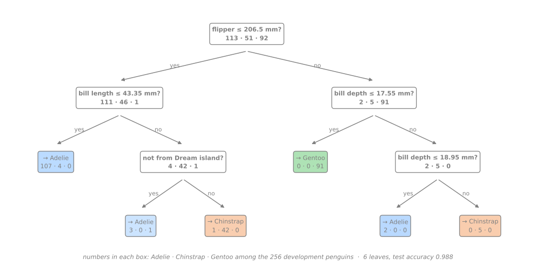
Rule 3 uses the island: in this dataset Chinstraps were only sampled on Dream, so "long bill on Dream" is a strong clue. It is a fact about where these birds were measured, not about the species, and a biologist reading the key would flag it; a model nobody reads would use it silently. Rules 5 and 6 rest on 2 and 5 birds, the kind of leaf the pruning rule tolerated but that deserves little trust. The importances confirm the reading: flipper length (0.548) and bill length (0.328) carry the key, and body mass and sex are never used. Remember the bias measured above; with 256 rows and 5 splits, these importances say "which questions the key asks", no more.
Step 10 — how stable is the key?
Predict. If another team measured similar penguins and ran the same recipe, would the key start with the same question? And would the predictions change as much as the questions?
rng = np.random.default_rng(0)
roots, preds = [], []
for b in range(100):
    idx = rng.integers(0, len(X_train), len(X_train))             # bootstrap resample
    m = DecisionTreeClassifier(random_state=0, **params).fit(X_train.iloc[idx], y_train.iloc[idx])
    roots.append((X.columns[m.tree_.feature[0]], round(m.tree_.threshold[0], 2)))
    preds.append(m.predict(X_test))
roots = pd.DataFrame(roots, columns=['feature', 'threshold'])
print(roots.groupby('feature')['threshold'].agg(['count', 'min', 'max']))
preds = np.array(preds)
disagree = np.mean([np.mean(preds[i] != preds[j]) for i in range(100) for j in range(i + 1, 100)])
print(f"two resampled keys disagree on {disagree:.1%} of the test penguins")
print(f"test penguins on which all 100 keys agree: {np.mean((preds == preds[0]).all(axis=0)):.1%}")
                   count     min     max
feature
culmen_depth_mm       12   16.05   16.40
culmen_length_mm      32   41.55   43.35
flipper_length_mm     56  202.50  207.50
two resampled keys disagree on 4.1% of the test penguins
test penguins on which all 100 keys agree: 73.3%
The same recipe (depth 3, ccp_alpha=0.01) applied to 100 bootstrap resamples of the development set produces keys that start with three different questions: flipper length in 56 of them, bill length in 32, bill depth in 12. Printed on a card, they would look like three different keys. Their predictions differ less than their structure, because on easy birds every key agrees: two keys disagree on 4.1% of the test penguins, and all 100 agree on 73.3% of them. Here is the practical meaning of instability: the specific questions of a tree are not a finding about penguins; they are one of several equally good ways to cut this sample. Read the rules as a working tool, not as biology, and do not be surprised if next season's data produces a different key.
Simulation: bagging by hand. Step 10 showed that keys trained on different resamples disagree. Turn that to your advantage: inside each fold of cv, fit 100 fully grown trees, each on a bootstrap resample of the fold's training part, and let them vote (the most frequent species among the 100 predictions). Compare with a single fully grown tree, on the same folds.
Solution
votes_acc, single_acc = [], []
for tr, va in cv.split(X_train, y_train):
    Xa, ya, Xv, yv = X_train.iloc[tr], y_train.iloc[tr], X_train.iloc[va], y_train.iloc[va]
    bag = np.random.default_rng(0)
    preds = []
    for b in range(100):
        idx = bag.integers(0, len(Xa), len(Xa))                    # one bootstrap resample of the fold
        preds.append(DecisionTreeClassifier(random_state=0).fit(Xa.iloc[idx], ya.iloc[idx]).predict(Xv))
    vote = pd.DataFrame(preds).mode(axis=0).iloc[0].to_numpy()     # the most voted species
    votes_acc.append(np.mean(vote == yv.to_numpy()))
    single_acc.append(DecisionTreeClassifier(random_state=0).fit(Xa, ya).score(Xv, yv))
print(f"one fully grown tree: {np.mean(single_acc):.3f} ± {np.std(single_acc):.3f}")
print(f"vote of 100 trees:    {np.mean(votes_acc):.3f} ± {np.std(votes_acc):.3f}")
print("per fold, vote - single:", np.round(np.array(votes_acc) - np.array(single_acc), 3))
one fully grown tree: 0.969 ± 0.016
vote of 100 trees:    0.976 ± 0.019
per fold, vote - single: [0.019 0.02  0.    0.    0.   ]
The vote of 100 trees scores 0.976, against 0.969 for a single tree: it wins on two folds, ties on the other three and never loses. The gain is small because on penguins one tree already makes few errors; the mechanism is the same as on Spambase in section 11 (from 0.895 to 0.950): the errors of trees trained on different resamples are partly independent, and the vote cancels part of them. You have just built most of a random forest; all that is missing is drawing at random the features each split may use, the subject of the next lesson.
To close the lesson. In one sentence each: (1) why did the key lose to the logistic regression, and what partly recovered it? (2) Why do keys trained on different resamples start with different questions? (3) Why does a vote of many trees err less than a single tree?
Your turn (advanced)
At home, with more time:
- Entropy in the grid. Add
'criterion': ['gini', 'entropy']to the grid of step 6. How many of the configurations within one standard deviation use entropy? Does the chosen key change? - A regression tree. On the California housing CSV (
pd.read_csv('https://raw.githubusercontent.com/hsandmann/biblio/refs/heads/main/ml/aula02/housing.csv')), predictmedian_house_valuefrom the numeric columns with aDecisionTreeRegressor. Tunemax_depthandmin_samples_leafwithKFold(5, shuffle=True, random_state=0)and compare the RMSE of the best tree with aLinearRegression. What is the largest value the tree can ever predict, and why? - Permutation importance. Compute
permutation_importance(key, X_test, y_test, n_repeats=30, random_state=0)(fromsklearn.inspection) and compare it with the impurity importances of step 9. Does the Dream island still matter? Does any feature the key does not use gain importance?
References
- Breiman, L.; Friedman, J. H.; Olshen, R. A.; Stone, C. J. Classification and Regression Trees. Wadsworth (1984) — CART: binary splits, Gini, regression trees, cost-complexity pruning and the one-standard-error rule. DOI
- Quinlan, J. R. "Induction of Decision Trees." Machine Learning 1, no. 1 (1986): 81–106 — ID3 and information gain. DOI
- Quinlan, J. R. C4.5: Programs for Machine Learning. Morgan Kaufmann (1993) — the successor of ID3, with gain ratio, continuous features, missing values and pruning.
- Morgan, J. N.; Sonquist, J. A. "Problems in the Analysis of Survey Data, and a Proposal." Journal of the American Statistical Association 58, no. 302 (1963): 415–434 — AID, the first regression tree. DOI
- Hyafil, L.; Rivest, R. L. "Constructing Optimal Binary Decision Trees is NP-Complete." Information Processing Letters 5, no. 1 (1976): 15–17 — why every practical algorithm is greedy. DOI
- Raileanu, L. E.; Stoffel, K. "Theoretical Comparison between the Gini Index and Information Gain Criteria." Annals of Mathematics and Artificial Intelligence 41 (2004): 77–93 — the two criteria disagree on about 2% of splits. DOI
- Strobl, C.; Boulesteix, A.-L.; Zeileis, A.; Hothorn, T. "Bias in Random Forest Variable Importance Measures: Illustrations, Sources and a Solution." BMC Bioinformatics 8 (2007): 25 — impurity importance favors features with many values. DOI
- Hastie, T.; Tibshirani, R.; Friedman, J. The Elements of Statistical Learning. 2nd ed., Springer (2009), section 9.2 — trees, impurity measures, pruning, instability. Free PDF
- Hopkins, M.; Reeber, E.; Forman, G.; Suermondt, J. "Spambase." UCI Machine Learning Repository (1999) — the e-mails used in this lesson (OpenML 44). DOI
- Gorman, K. B.; Williams, T. D.; Fraser, W. R. "Ecological Sexual Dimorphism and Environmental Variability within a Community of Antarctic Penguins (Genus Pygoscelis)." PLoS ONE 9, no. 3 (2014): e90081 — the lab's penguins (OpenML 42585). DOI
Quiz
The quiz covers the fundamental approach.