Machine Learning · Insper

Decision Trees

Advanced approach

Where trees shine, where they fail, and why they became the raw material of ensembles

The path of this part

Measure the splitimpurity, not errors; variance for regression
Prune after growingcost-complexity pruning and the choice of α
Face the instabilitya small change in the data, a different tree
Strengths and limitsscaling, staircases, NaN, importance

Each stage answers one question: what should a split measure? → how much of a grown tree should we keep? → how far can one tree be trusted? → when is a tree the right tool?

Stage 1 · what should a split measure?

Why not simply count errors?

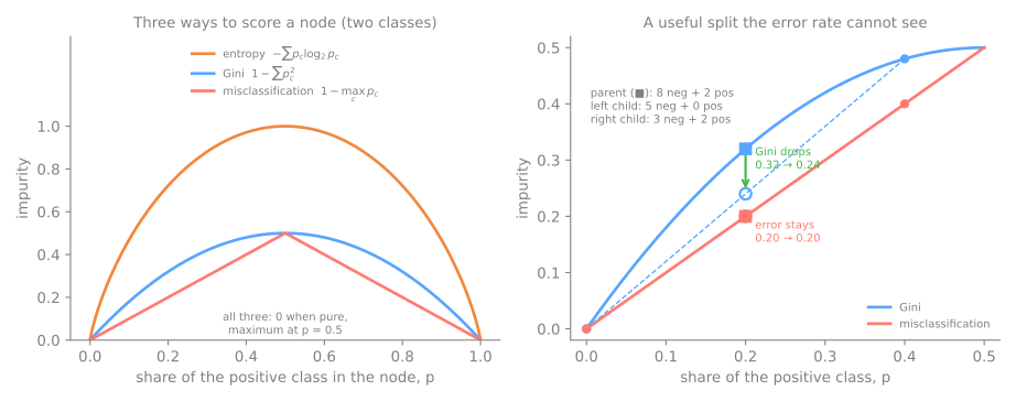
Entropy, Gini and error rate; a split where the error rate does not move and Gini falls

Parent: 8 negatives, 2 positives. Split: 5 + 0 and 3 + 2. Both children still predict "negative": error rate 0.20 → 0.20.
Yet one child is pure and the positives are concentrated: Gini 0.32 → 0.24.

Gini and entropy are strictly concave: they reward progress before the prediction changes. That is what makes the greedy search work.

Regression trees

A leaf predicts the mean; the impurity is the MSE around it (the variance of the target in the node).

\[ I(\text{node}) = \frac{1}{n}\sum_{i \in \text{node}} (y_i - \bar y)^2 \]

Eight flats: mean R$ 2.362 thousand, MSE 0.7873.
area ≤ 67.5: R$ 1.720 thousand for the five small ones, R$ 3.433 thousand for the three large ones; weighted MSE 0.0993.

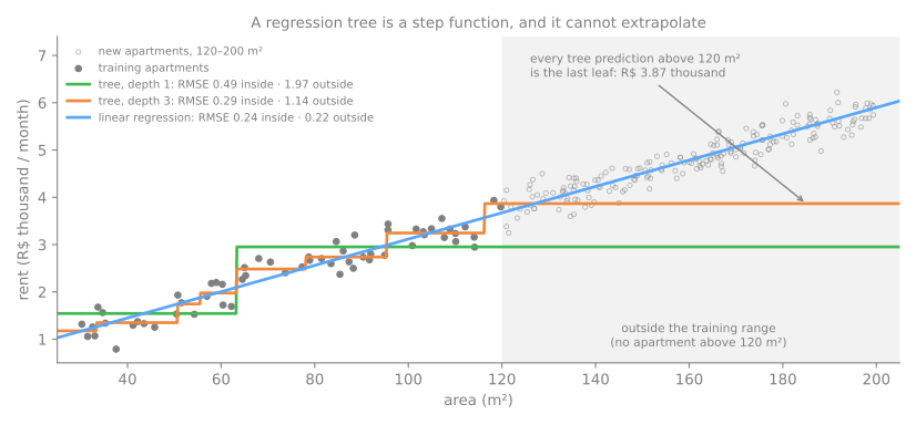
A single question removes 87% of the variance. Same algorithm, another impurity.

A staircase that cannot extrapolate

Depth-1 and depth-3 trees and a line fitted to rents; above 120 m² the trees go flat

With $L$ leaves, at most $L$ values. Above 120 m², the depth-3 tree says R$ 3.87 thousand for any size: RMSE outside the range 1.14, against 0.22 for the line.

Stage 2 · how much of a grown tree should we keep?

Post-pruning: grow, then cut back

\[ R_\alpha(T) = R(T) + \alpha\,|T| \qquad \alpha_{\text{eff}}(t) = \frac{R(t) - R(T_t)}{|T_t| - 1} \]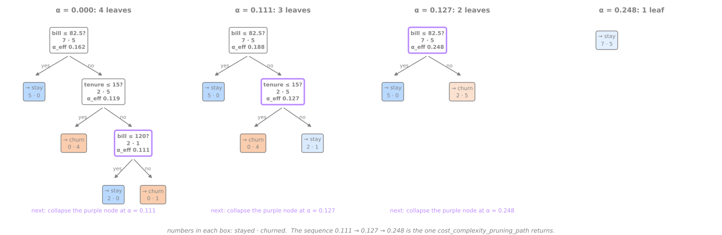

Weakest-link pruning of the churn tree in four stages

Each step collapses the node with the smallest $\alpha_{\text{eff}}$: 0.111 (the split that isolated J) → 0.127 → 0.248. It is the sequence cost_complexity_pruning_path returns.

Pruning on Spambase

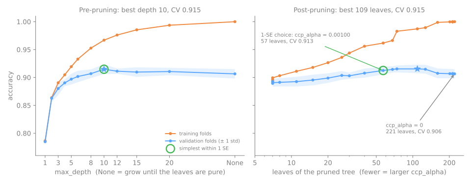
Training and validation accuracy by depth and by number of leaves when pruning

Unpruned: 221 leaves, 0.906. Best $\alpha$: 109 leaves, 0.915.
One-standard-error rule (Breiman et al., 1984): 57 leaves, 0.913 — a quarter of the tree.

Pruning buys little accuracy here; its real win is size: just as accurate and far easier to read.

Stage 3 · how far can one tree be trusted?

Instability: a small change, a different tree

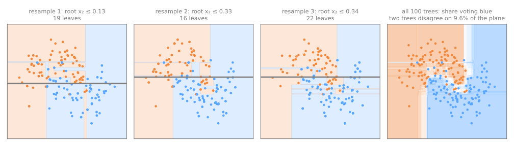
Three trees from bootstrap resamples with different boundaries

50 bootstrap resamples of Spambase:

the root changes: $ in 29, ! in 19, two other words once each;
136 to 186 leaves;
accuracy 0.895 on average, yet two trees disagree on 11.8% of the e-mails.

Letting the 50 vote gives 0.950, better than the best single tree (0.919). Instability is a tree's flaw and the ensemble's raw material.

Stage 4 · when is a tree the right tool?

What trees do not need

Scaling

A split only uses the order. Standardizing: the same predictions on 100% of the test set. log1p: 99.3% (only the thresholds between values move).

Interactions

"Tenure matters when the bill is high": the tree says it by nesting questions, without a product feature.

Imputation

Since scikit-learn 1.3, NaN goes straight in: each split learns which way to send missing values.

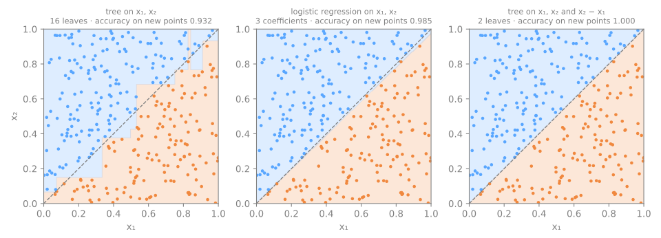
Where they struggle: diagonals become staircases

A diagonal boundary approximated by steps; logistic regression and a tree given the x2 − x1 feature

16 leaves and 0.932 for what the logistic regression says with one line (0.985). With the feature $x_2 - x_1$, 2 leaves and 1.000: feature engineering helps a tree more than any hyperparameter.

Feature importance, and its bias

feature_importances_ adds up the impurity decrease of each feature's splits, on the training data.
A column of random numbers ranks 12th of 59, ahead of 46 real features; a random coin ranks 41st.
Features with many values offer many thresholds; one of them separates a few noisy rows by chance (Strobl et al., 2007).

To measure importance for real: permutation on held-out data (next lesson) or SHAP (Explainability).

Practical profile

Strengths	readable rules; no scaling; automatic interactions; accepts `NaN`; fast
Weaknesses	overfits without pruning; unstable; staircases for diagonals; cannot extrapolate; biased importance; coarse probabilities
Use when	the model must be read, audited or applied by hand

One tree, rarely; many trees, all the time: random forests (many deep trees, averaged) and gradient boosting (many shallow ones, added up).

Advanced lab · about 35 min, in pairs

The final key, and what it is worth, steps 6 to 10

Same notebook, same session: the steps use X, X_train, y_train, cv and cv_report.
Tune depth, leaves and pruning; compare with logistic regression and k-NN on the same folds; test once; measure how stable the key is.
Notebook on Colab (in Portuguese), from step 6.
Simulations: give the tree the diagonal (step 7) and bagging by hand (step 10).

Pace: steps 6 and 7 and the first simulation in 15 min; steps 8 and 9 in 10 min; step 10 and the second in 10 min.