Machine Learning · Insper

Dimensionality Reduction

Advanced approach

How much a map of PCA (principal component analysis), t-SNE (t-distributed stochastic neighbor embedding) or UMAP (uniform manifold approximation and projection) can be trusted, measured

Where the fundamental part left off

PCA: the eigenvectors of the covariance; the eigenvalue is the variance kept; it has transform.
t-SNE and UMAP: maps that keep each point's neighbors; sizes, distances between groups and axes mean nothing.
Seven forbidden statements, given as rules.

A plot is a hypothesis. This part turns the rules into numbers: a score for a map, a null comparison, a seed test, held-out points.

The path of this part

PCA's pitfallsunits, leakage, target, factors, one-hot
Score a maptrustworthiness; Isomap and the manifold family
Stress-test t-SNEgroups in noise; axes and seeds
New points, every scaleUMAP's transform; trustworthiness at every k

Each stage answers one question: how can a PCA say something false? → how do we score a map? → does t-SNE find what is not there? → can the map take new points, and at which scale is it good?

Stage 1 · how can a PCA say something false?

Five PCA pitfalls

Not standardizing columns in different units: you measure the unit (wine: PC1 = proline, 99.8%).
Fitting before the split: the test rows shape the projection.
Assuming high-variance components are the useful ones for prediction: PCA never looks at the target.
Reading components as real-world factors: signs are arbitrary, and close eigenvalues allow any rotation.
PCA on one-hot columns without thinking: a 0/1 column with share \(p\) of ones has variance \(p(1-p)\), so rare categories vanish.

None of the five produces an error message. The code runs, the shapes are right, and the conclusion is false.

Stage 2 · how do we score a map?

A score for a map: trustworthiness

Of the \(k\) nearest neighbors of each point on the map, how many were really neighbors in the original space? Intruders cost more the farther away they really were. 1 = no intruders.

Predict. A map that places the points at random: what does it score, 0 or something else?

random map

≈ 0.5

the floor, not 0

PCA on the Swiss roll

0.810

layers land on top of each other

Isomap

0.976

walks a 10-neighbor graph: unrolls the sheet

One bet, many methods

The bet: Euclidean distance is only trustworthy locally. MDS = multidimensional scaling; LLE = locally linear embedding.

method	idea	status today
Kernel PCA	PCA in a kernel's feature space	choose the kernel; \(O(n^2)\) memory
MDS	keep all pairwise distances	historical basis; crowding
Isomap	MDS on graph (geodesic) distances	short-cut edges between layers
LLE / Laplacian eigenmaps	local reconstructions / graph Laplacian	ancestors of UMAP
t-SNE	match neighbor distributions	visualization standard since 2008
UMAP	fuzzy graph + optimized layout	current standard at scale
Autoencoder	a network learns map and inverse	reversible; bridge to deep learning

Stage 3 · does t-SNE find what is not there?

t-SNE finds groups in noise

200 points of uniform noise in 10 columns. A k-means clustering scored by its silhouette (near 1 for separated groups, near 0 when there are none) says how "groupy" a set of points looks.

Predict. The noise itself scores 0.09. Its t-SNE map: higher, lower or the same?

	best silhouette	trustworthiness
10-column noise itself	0.09
its t-SNE map, perplexity 30	0.38	0.86
4-column noise, t-SNE map	0.43	0.97

A good trustworthiness does not certify the structure: noise has local neighborhoods too. The cure is a null comparison: shuffle each column independently, rerun, compare.

Axes and runs

The loss depends only on distances on the map: rotating or mirroring it changes nothing. Digits, random initialization, seed 0 against seeds 1, 2, 3:

horizontal axes |correlation|

1.0, 0.0, 0.1

seed 2 came out rotated a quarter turn

neighbors in common

90%, 94%, 85%

on noise: only 47%

The neighborhoods are real; the orientation is not. init="pca" (the default) makes the map reproducible, which is not the same as stable.

Stage 4 · can the map take new points, and at which scale is it good?

UMAP places new points, measured

The digits: UMAP fitted on 80% of the images, then reducer.transform on the other 20%.

Predict. How often will a new image land next to a training image of its own digit?


hasattr(PCA(), "transform")    # True
hasattr(TSNE(), "transform")   # False
reducer = umap.UMAP(n_neighbors=15, min_dist=0.1, random_state=0).fit(X_tr)
E_te = reducer.transform(X_te)                 # 360 new images, same map

new image next to its own digit

96.4%

t-SNE

no transform: adding points means recomputing the whole map, which moves the old points too

PCA vs t-SNE, side by side

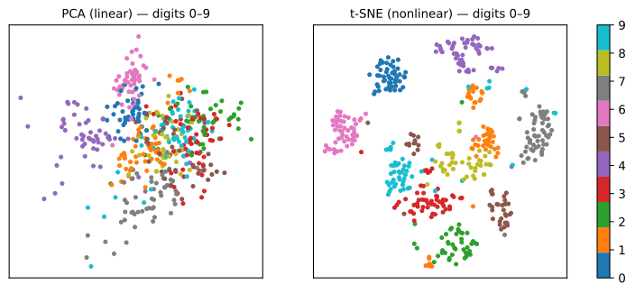
Digits: PCA overlaps the classes (0.830), t-SNE separates them (0.992) but splits the 1s; Swiss roll: PCA smears (0.810), t-SNE cuts the sheet into pieces (0.976)

Trustworthiness on the digits, for neighborhoods of size \(k\):

	k=5	k=30	k=100
PCA	0.830	0.830	0.835
t-SNE	0.995	0.985	0.963
UMAP	0.989	0.983	0.961

t-SNE splits the 1s into islands and cuts the roll into pieces. No winner until you say which scale you care about.

Summary: a reduction needs a number

to claim that...	measure
\(k\) components keep almost everything	cumulative explained variance; reconstruction error
the map keeps each point's neighbors	trustworthiness, at more than one \(k\) (random ≈ 0.5)
the groups on the map exist	a clustering in the original space; a null comparison
the picture is stable	neighbor overlap across seeds, perplexities, samples
the map works on new data	`transform` (PCA, UMAP), scored on held-out rows

A plot is a hypothesis, not a result.

Advanced lab · about 30 min, in pairs

Putting numbers on the maps, steps 5 to 8

Same notebook and session as the fundamental lab: X, y, X_new, maps, reducer from steps 1 to 4.
Steps: 5. score the maps with trustworthiness · 6. perplexity · 7. UMAP: n_neighbors, min_dist, new images · 8. test a forbidden statement.
At every step, answer the Predict before running.
Simulations: a map that knows nothing (step 5) and t-SNE has no transform, so start over (step 7).

Pace: step 5 and the first simulation in 8 min; step 6 in 5 min; step 7 and the second simulation in 12 min; step 8 in 5 min.