Machine Learning · Insper

Dimensionality Reduction

Fundamental approach

A few new columns that keep what matters: the curse of dimensionality, PCA (principal component analysis) by hand, and the maps of t-SNE (t-distributed stochastic neighbor embedding) and UMAP (uniform manifold approximation and projection)

Why reduce? The reason picks the method

goal	what the method must deliver	typical method
see the data	a 2-D or 3-D picture; local fidelity is enough	t-SNE, UMAP
compress / speed up	reconstruction, and a transform for new data	PCA
remove noise / collinearity	drop the low-variance directions	PCA
feed another model	an honest `fit`/`transform`, no leakage	PCA (almost always)

Mixing up these reasons is behind most misuse of these methods.

The path of this part

The cursedistances lose their contrast
PCA by handcenter, covariance, eigenvectors, project
Scale, choose k, rebuildunits, explained variance, reconstruction error
Bend: t-SNE and UMAPwhere PCA runs out; neighbors instead of variance
Read and chooseseven forbidden statements; the goal decides

Each stage answers one question: why do many columns hurt? → which direction keeps the most variance? → does the unit matter, and how many components? → how do we map a curved structure? → what can a map say, and which method fits which goal?

Stage 1 · why do many columns hurt?

The curse of dimensionality

Take random points in the unit cube and look at the distances between them.

Predict. In 1,000 dimensions, how much farther is a point's farthest neighbor than its nearest: 40 times, 10 times, or about 10%?

Simulator: distances in \(d\) dimensions

Push \(d\) up and watch the histogram of distances collapse into a spike.

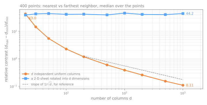
Relative contrast, measured

\((d_{\max} - d_{\min})/d_{\min}\), median over 400 points:

\(d\)	noise columns	2-D sheet in \(d\) columns
2	42.97	39.23
10	2.27	41.51
100	0.39	45.88
1000	0.11	44.24

Relative contrast against the number of columns: noise falls from 43.0 to 0.11; the rotated 2-D sheet stays between 39 and 46

Concentration is not caused by the number of columns: the rotated sheet has 1,000 columns and does not move. What hurts is columns that carry no information. The real question: how many directions actually vary?

Stage 2 · which direction keeps the most variance?

PCA: the directions of maximum variance

Centered data \(X\); covariance \(C = \frac{1}{n-1} X^\top X\).

\[ w_1 = \arg\max_{\|w\|=1} w^\top C\, w \qquad \text{EVR}_k = \frac{\lambda_k}{\sum_j \lambda_j} \]

\(w_1\) is the eigenvector of \(C\) with the largest eigenvalue \(\lambda_1\); the next is orthogonal to it, and so on.
\(\lambda_k\) is the variance captured by component \(k\); EVR is the explained variance ratio.

By Pythagoras, the part of each point along the line plus the part perpendicular to it is fixed: maximum variance = minimum reconstruction error.

PCA by hand, step by step

Five points: (2, 4), (4, 2), (5, 5), (6, 8), (8, 6). Predict. Where will PC1 point, and what share of the variance will it keep? Then step through center → covariance → eigenvalues → eigenvector → project → reconstruct.

The same in code, and two details

np.linalg.eigh returns the eigenvalues in ascending order: the best direction comes last. Forgetting to sort is a silent bug.
scikit-learn's PCA agrees: explained_variance_ratio_ = [0.8, 0.2].
Signs are arbitrary: \(w\) and \(-w\) are both eigenvectors; read relative signs inside a component, never the absolute sign.
New points need no refitting: \((9,7) - (5,5) = (4,2)\), and \((4+2)/\sqrt2 = 4.243\), exactly pca.transform.

This is what lets PCA sit inside a pipeline. t-SNE cannot do it.

Simulator: rotate the line

Predict. As you turn the line, at how many angles does the captured variance peak? Then press find PC1.

Stage 3 · does the unit matter, and how many components?

The scaling question

Wine: 13 chemical measurements of 178 wines. Proline has standard deviation 314.9; hue is around 1.

Predict. On the raw columns, what will PC1 be?

	variance ratio of PC1, PC2, PC3	largest weights in PC1
raw columns	0.998, 0.002, 0.0	proline 1.000
standardized	0.362, 0.192, 0.111	flavanoids, total phenols, OD280

99.8% is not a discovery about wine: it is a measurement of the unit of proline.

Does it matter downstream?

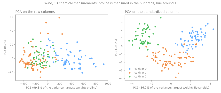
Wine on PC1 and PC2: raw, the cultivars overlap; standardized, they form three separate groups

A k-NN classifier (k-nearest neighbors) that sees only the two PCA coordinates, scored on 30% of the wines:

raw → PCA(2)

0.722

scaled → PCA(2)

0.926

Standardize when columns are in different units; not blindly when they share a unit and their variance means something (the pixels of an image). And keep PCA inside the pipeline.

Choosing \(k\): 64 pixels of digits

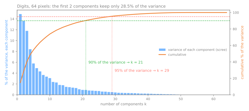
Scree bars of the 64 digit components and the cumulative explained variance; 2 components keep 28.5%, 90% needs 21, 95% needs 29

2 components keep 28.5%: a 2-D PCA picture shows less than a third.
90% needs 21, 95% needs 29, 99% needs 41.
PCA(n_components=0.95) searches for you.

Criteria, most trusted first: a cumulative-variance threshold; the elbow (subjective); downstream performance on validation data; Kaiser's rule (fragile).

Reconstruction: what \(k\) components keep

\(k\)	kept	error / image	discarded \(\lambda\)
1	14.9%	1022.6	1022.6
2	28.5%	858.9	858.9
10	73.8%	314.5	314.5
29	95.5%	54.3	54.3
64	100.0%	0.0	0.0

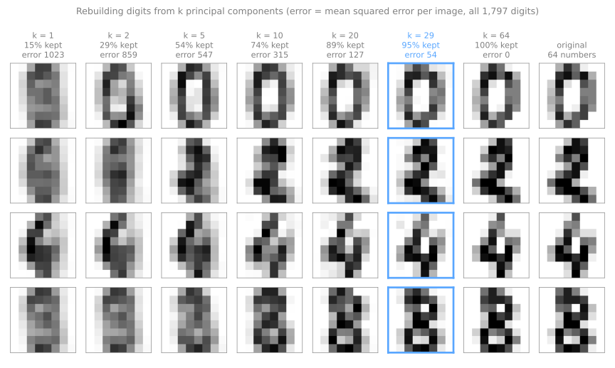
The two last columns are the same number: the error is the sum of the discarded eigenvalues. Hence compression and denoising.

Simulator: rebuild an image from \(k\) components

Predict. How few components does your eye need before it stops objecting?

Stage 4 · how do we map a curved structure?

Where PCA runs out

PCA can only rotate and project: it moves the axes, never bends them.

The Swiss roll: a 2-D sheet rolled up in 3-D. Two points on opposite layers are close in straight line, far along the sheet.

Predict. Project the roll with PCA. What happens to the colors of the two layers?

Simulator: the Swiss roll

Tick mark a pair of points, then project with PCA. Euclidean distance goes through the empty space; geodesic distance walks along the sheet.

t-SNE in three steps

Neighborhoods in the data: a Gaussian around each point, its width tuned per point to a perplexity ("effective number of neighbors"). Dense and sparse regions get different widths.
Neighborhoods on the map: a Student-t, with heavy tails, to make room in 2-D. Side effect: distances between groups stop meaning anything.
Minimize the Kullback–Leibler divergence \(\text{KL}(P\,\|\,Q)\): true neighbors drawn far apart are expensive; far points drawn close are almost free.

What is close in the data is usually close on the map. What is close on the map may not be close in the data.

Simulator: real t-SNE, in your browser

Try. Run it on uniform noise; change only the perplexity; compare groups of different sizes.

What a t-SNE map does not tell you, measured

	data	t-SNE
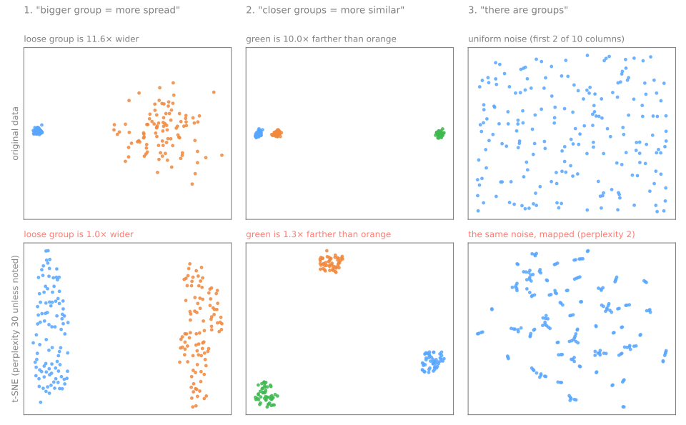
how many times wider the loose group is	11.6	1.0
how many times farther the far group is	10.0	1.3

Original data and t-SNE: groups 11.6 times different in width come out the same size; a group 10 times farther comes out 1.3 times farther; noise becomes clumps

Not bugs, the design: the per-point width equalizes dense and sparse groups, and the heavy tail makes "far" and "very far" cost the same.

Perplexity changes the picture

perplexity	distance ratio
2	3.3
5	1.1
30	1.3
100	7.0

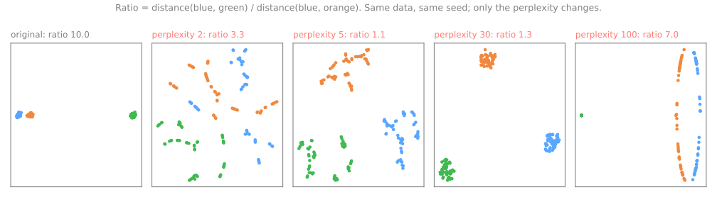
The three groups at perplexity 2, 5, 30 and 100: fragments at 2 and 5, equidistant at 30, the far group pushed away at 100

At 2 and 5 every group shatters into fragments that do not exist. There is no "right" perplexity: usually 5–50, smaller than the smallest group you want to see.

Run several and trust only what persists. Report the perplexity like a random seed.

UMAP: a graph of neighbors

Each point is linked to its n_neighbors nearest points, with fuzzy weights; no point is left isolated.
The weights are merged into one symmetric fuzzy graph.
A 2-D layout by stochastic gradient descent: edges attract, sampled random points repel; an explicit penalty for putting distant points close.

`n_neighbors` (15)

the scale at which Euclidean distance is trusted: local detail against global structure

`min_dist` (0.1)

how tightly points are packed: cosmetic, not structural

UMAP has transform: fit on 80% of the digits, 96.4% of the new images land next to an image of the same digit.

Stage 5 · what can a map say, and which method fits which goal?

The comparison table

	PCA	t-SNE	UMAP
nature	linear, deterministic	nonlinear, stochastic	nonlinear, stochastic
local structure	weak	very good	very good
global structure	best (variance)	weak	moderate
group distances / sizes	yes / yes	no / no	partly / no
`transform` new data	yes, trivial	no	yes
key hyperparameters	\(k\), scaling	perplexity, iterations	`n_neighbors`, `min_dist`
preprocessing for a model	recommended	not advised	with care, in the pipeline

Seven forbidden statements about a t-SNE/UMAP plot

"This group is bigger, so it varies more." (11.6× in the data, 1.0× on the map)
"These two groups are close, so they are similar." (10× in the data, 1.3× on the map)
"There are 5 groups in the data." There are 5 blobs on the plot.
"The horizontal axis represents X." Rotation and reflection are arbitrary.
"I ran it once and saw this." Vary seed, perplexity, sample.
"I used the 2 t-SNE components as features." No honest transform.
"I ran t-SNE on the whole dataset and then split." Leakage.

A plot is a hypothesis, not a result. A claim needs a number: reconstruction error, trustworthiness at several scales, a null comparison, a downstream model.

Choosing a method

It will feed another model, or you need reversibility → PCA. Full stop.
You want to look at the data to form hypotheses, up to a few thousand points → t-SNE or UMAP, with PCA first if \(d\) is large.
\(n\) is large, or you must project new data onto the same map → UMAP.
You need reliable global structure in one picture → none is ideal: show PCA and t-SNE/UMAP.

Summary

Many columns hurt only when they carry no structure; ask how many directions actually vary.
PCA = eigenvectors of the covariance, sorted by eigenvalue; \(\lambda_k\) is the variance along component \(k\).
Kept and dropped share one budget: explained variance chooses \(k\); the reconstruction error is the sum of the dropped eigenvalues.
Standardize columns in different units, not pixels; fit PCA inside the pipeline.
t-SNE and UMAP keep neighbors, nothing else; only PCA and UMAP place new points.

symptom	what to do
PC1 explains 99% and is a single column	standardize, then refit
tidy groups on a t-SNE map	validate them in the original space
a classifier fed with 2 t-SNE coordinates	PCA (or UMAP) inside the pipeline

Fundamental lab · about 30 min, in pairs

Mapping handwritten zip codes, steps 1 to 4

USPS (US Postal Service) digits: 9,298 handwritten digits from envelopes, 16×16 = 256 columns; we map a sample of 1,500.
Download the lab notebook and open it in Jupyter or Colab; in Colab, run !pip install umap-learn first.
Steps: 1. load a sample · 2. how many dimensions? · 3. compression and reconstruction error · 4. three maps of the same images.
At every step, answer the Predict before running.
Simulations: standardize the pixels anyway (step 2) and compress images the PCA never saw (step 3).

Pace: step 1 in 5 min; step 2 and the first simulation in 10 min; step 3 and the second in 10 min; step 4 in 5 min.