The path of this part
- Spot redundancyfeatures that say the same thing; leaked columns
- Condition on a third variablecorrelation is not causation; Simpson's paradox
- Judge the odd valuesrules that disagree; error or rare but real
- Face the ceilingcapped values, censored targets
Redundant features
- The four counts (rooms, bedrooms, population, households) correlate at 0.86 to 0.98: all measure how big the district is.
- Iris: petal length and width, \(r = 0.963\).
- Not an error, but worth writing down: linear models get unstable coefficients; dimensionality reduction exploits it; for the counts, divide by the size.
Correlation is not causation
- Income and house value: \(r = 0.69\). Raising a district's income does not raise its prices, nor the reverse.
- Both respond to a third thing: the demand for living there (jobs, coast, schools).
- Ice cream sales and drownings correlate through summer.
Simpson's paradox: kidney stones
| success rate | treatment A | treatment B |
|---|---|---|
| small stones | 0.931 | 0.867 |
| large stones | 0.730 | 0.688 |
Overall: A 0.780, B 0.826. A loses: \(273/350\) for A.
A was mostly given to large stones (263 of 350), which are harder to treat. The size of the stone is a confounder: it influences both the choice of treatment and the success.
The same trap in the housing data
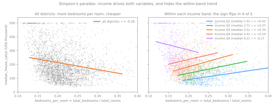
Share of rooms that are bedrooms vs value:
overall \(r = -0.256\); within income bands Q1–Q4, +0.24 to +0.42.
Income drives both (\(r = -0.616\) with the bedroom share).
On real data the rules disagree
population, IQR
population, \(|z| > 3\)
log(population), IQR
A long right tail puts many ordinary large districts beyond the fences at 1.5 IQR (interquartile range: \(Q_3 - Q_1\)).
Error, or rare but real?
age = 190in a customer table: a typing error → fix it or set it to missing.- The owner's salary of 26: real → keep it; prefer robust statistics (median, quantiles, log).
- In between: values that are correct but mean something different.
Capped (censored) values
value at 500,001
age at 52
income at 15.0001
Top-coding: 500,001 means "at least 500,000"; the true value was lost. The capped districts are not random: mean income 7.83 against 3.87 overall.
How to spot a cap, and what it does
histogram
a spike at the very edge, taller than its neighbors (with enough bins)
scatter plot
a horizontal line: 965 districts at 500,001
the maximum
shared exactly by many rows: 1,273 districts at age 52
- A model trained on these values learns that no district is worth more than about 500,000.
- Relationships flatten at the top: income against value seems to level off after an income of about 8, partly because of the cap.
Summary
| symptom | what is happening | what to do |
|---|---|---|
| two features with \(|r|\) above 0.9 | they measure the same thing | keep one, or make a ratio |
| one feature almost perfect at predicting the target | maybe the target in disguise | find out how it was produced |
| a correlation that changes sign within groups | a third variable drives both | report it within the groups |
| the IQR rule flags thousands of rows | a long tail, not errors | look at them; try a log or a ratio |
| many rows share the maximum exactly | the column is capped | document it; state the range the model covers |
From the map to a data card, steps 8 to 11
- Same notebook, same session: continue from step 8.
- The map (latitude against value, band by band) → counts and ratios → outliers and odd districts → the written data card: facts, problems to fix, hypotheses to test.
- At every step, answer the Predict before running.
- Simulations: give location a direction (step 8) and clean every column with the IQR rule (step 10).
Pace: step 8 and the first simulation in 10 min; step 9 in 5 min; step 10 and the second simulation in 10 min; step 11 in 5 min.