Machine Learning · Insper

Explainability

Advanced approach

When do explanations mislead, and how do you check them?

Three tools, one hidden assumption

permutation importance

shuffle one column, keep the others

partial dependence (PDP)

set one feature to $v$ in every row, keep the others

SHAP (SHapley Additive exPlanations)

fill the missing features from a background, one by one

All three change a feature while holding the others fixed, whether or not that combination exists.

When features move together, "holding the others fixed" splits their credit and creates rows that do not exist. This part measures both, meets a second local method, LIME, and ends with a checklist.

The path of this part

Correlated featuresshared credit and impossible rows
Off the mapa PDP averaged over places that do not exist
Another local answerLIME, and how wide "local" is
Estimates, not certificatesthree rankings, choices inside, a checklist

Each stage answers one question: what happens to an importance when features are correlated? → what does a PDP average over? → why do two local methods disagree? → how much should we trust an explanation?

Stage 1 · what happens to an importance when features are correlated?

Correlated features (1): shared credit

Add an exact copy of income and refit the random forest. Predict. Each copy's permutation importance falls to 0.196. What does shuffling both together give?

	MDI	perm. on test
income alone	0.516	0.754
income	0.262	0.196
income_copy	0.259	0.196
both shuffled together		0.748

MDI: mean decrease in impurity, the importance trees compute on their training splits.

Shuffle one copy and the trees that split on the other still work.

Together the two copies get 0.392, half of what the information is worth.

A "useless" feature may just have a substitute: permute correlated groups together.

Correlated features (2): impossible rows

Latitude and longitude: correlation −0.92, because California is a diagonal strip.
Shuffle latitude alone: a San Francisco longitude gets a San Diego latitude, a point in the Pacific.

45%

of the shuffled districts are more than 0.25° (about 25 km) from any real one

The model never saw such places. Part of the 1.330 measures latitude; part measures how badly the model behaves off the map.

That is why shuffling latitude "cost" more than the whole R² of 0.825. Fix: treat the correlated pair as one feature, "location".

Stage 2 · what does a PDP average over?

The extrapolation trap

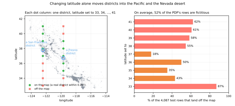
Map of California districts with the points a latitude PDP creates; most moved copies fall in the Pacific or the desert

latitude set to	33°	35°	37°	39°	41°
rows off the map	87%	35%	18%	58%	62%

The partial dependence plot (PDP) value at 33° is mostly the model's guess about places that do not exist. Check the individual conditional expectation (ICE) curves and the data's range; plot correlated pairs jointly; accumulated local effects (ALE) plots avoid this (Apley & Zhu, 2020).

Stage 3 · why do two local methods disagree?

LIME: a linear model around one row

perturb: thousands of points around the row
predict: ask the black box about each
weight: the closer, the heavier (kernel width $w$)
fit a weighted linear model

San Francisco	by hand	`lime`
income	42.1	42.0
occupancy	−49.9	−48.9
latitude	−89.3	−91.8
longitude	−53.6	−55.5

LIME: Local Interpretable Model-agnostic Explanations (Ribeiro, Singh & Guestrin, 2016). The coefficients are slopes, in $1,000 per standard deviation.

SHAP or LIME? They answer different questions

Predict. Same district, same feature: SHAP gives income +2.6, LIME gives +42.1 per standard deviation. Which one is wrong?

SHAP

how much does this district's actual income move its prediction away from the average? Its income is close to average: not much.

"why is this house expensive?"

LIME

what would happen if income changed? The local slope, which is steep.

"what would change the price?"

KernelSHAP is LIME run on coalitions, with one particular kernel and no regularization: that choice makes the regression return Shapley values.

How local is "local"?

width	0.5	1.0	2.12	5.0	std, 5 seeds
income	54.7	54.8	42.1	38.2	1.5
house_age	−9.9	1.3	1.3	1.0	1.3
occupancy	−71.0	−67.4	−49.9	−45.0	0.9

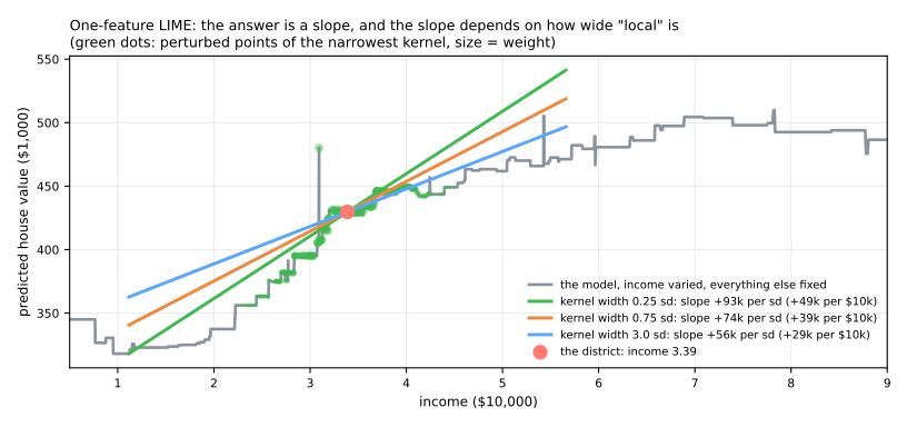
One-feature LIME: the model's staircase curve of price against income, and three local lines with slopes +93k, +74k and +56k

The seeds matter little (std: standard deviation across 5 seeds); the kernel width matters a lot, and house_age even changes sign. The default $0.75\sqrt{d} = 2.12$, with $d = 8$ features, is a convention, not a law.

Stage 4 · how much should we trust an explanation?

Three rankings, three questions

MDI

income first (0.567)

what did training use?

permutation

latitude first, a drop larger than 1, inflated by impossible rows

what does the score need?

mean |SHAP|

latitude first, 76.6 against 44.2 for income, in $1,000

how far does each feature move the predictions?

Choose the question before the method.

Explanations are estimates, with choices inside

choices measured in this lesson

the background sets SHAP's base value
the kernel width changes LIME's slopes
correlated features split their credit arbitrarily
permutation and PDP query impossible rows

they can even be gamed

Slack et al. (2020) built models that discriminate on real inputs while showing innocent explanations to LIME and SHAP, which probe them with off-distribution points.

Treat an explanation as evidence to be checked, not as a certificate.

A checklist for explaining a model

Try an interpretable model first; if it is as good on the same folds, use it.
Compute importances on held-out data.
Find correlated groups and permute or explain them together.
Look at ICE curves, not only the PDP; check that the plotted values are inside the data.
Use SHAP for local explanations; state the background you used.
When a feature dominates, ask when is this value recorded? (leakage).
Never read an explanation as a causal claim.

Advanced lab · about 25 min, in pairs

A protected attribute and a planted leak, steps 8 and 9

Same notebook, same session: continue from step 8 (if the session dropped, run steps 1 to 7 first).
Step 8: does the forest need personal_status? Retrain without it and compare the AUC (area under the receiver operating characteristic curve); then ask how many applicants it moves.
Step 9: plant a leak (collection letters, sent after a loan goes bad) and watch whether cross-validation or the explanations catch it.
Simulations: whom does personal_status push up? (step 8) and a subtler leak (step 9).
Lab notebook, for Jupyter or Colab.

Pace: step 8 and its simulation in 12 min; step 9 and its simulation in 13 min.