A good prediction nobody can read
- Random forests, gradient boosting and neural networks won the last lessons.
- A boosted ensemble of 200 trees predicts well, but "why this number?" has no answer you could write on a page.
global
which features does the model rely on, overall?
local
why did it make this prediction for this row?
Why explain a model?
debugging
a model that looks too good usually is: a leaked column shows up at the top of every importance ranking
trust
a doctor, a credit analyst or a judge will not act on a number they cannot question
regulation
Brazil's General Data Protection Law (LGPD, Lei 13.709/2018, art. 20): the right to ask for a review of automated decisions, with "clear and adequate information" about the criteria; Europe's General Data Protection Regulation (GDPR, art. 22) points the same way
science
sometimes the model is a tool to learn about the world, and the explanation is the result
The toolbox of this part
| method | question it answers | scope |
|---|---|---|
| coefficients, tree rules | the model itself | global |
| impurity importance (MDI, mean decrease in impurity) | which features did the training splits use most? | global, trees |
| permutation importance | how much does the score depend on each feature? | global |
| partial dependence plot (PDP) | how does the average prediction change with one feature? | global |
| ICE curves (individual conditional expectation) | ... and for each row? | local, many rows |
| SHAP values (SHapley Additive exPlanations) | how much did each feature move this prediction from the average? | local → global |
Model-specific methods read the internals; model-agnostic ones only call predict. LIME, a second local method, is in the advanced approach.
The path of this part
- Readable firstcoefficients, tree rules, the price of readability
- What matterspermutation importance, on held-out data
- With what shapepartial dependence and ICE curves
- Why this predictionShapley values, SHAP waterfalls and beeswarms
- Read with carenot causation; right for the wrong reasons
First: do you need a black box?
Three candidates on the same five folds, from fully readable to not readable at all.
Readability has a price, here
linear regression
tree, depth 3
gradient boosting
What the readable models say
eight coefficients
$10,000 more income → +$44,140 (with the others fixed); one degree north → −$41,300.
rooms −11.65 and bedrooms +63.55 have opposite signs: they are correlated (0.85), so "one more bedroom at a fixed number of rooms" means converting a room.
eight rules
Anyone can follow a district down the tree:
income above $78,000 → $457,900.
model is the black box: 200 trees with up to 16 leaves each. The rest of the lesson opens it.Permutation importance: shuffle one column
- Take held-out data and the model's score on it.
- Shuffle one column: its values stay, its link with the target and with the rest of each row breaks.
- Measure the drop in the score. Repeat for every column (Breiman, 2001).
for col in X_test.columns:
    X_perm = X_test.copy()
    X_perm[col] = rng.permutation(X_perm[col].to_numpy())
    drops[col] = base - r2_score(y_test, model.predict(X_perm))
Permutation importance, by hand
4,087 held-out districts, R² = 0.825 with nothing shuffled; each column shuffled 5 times. Predict. Can shuffling one column cost more than 0.825?
Two rankings of the same model
| permutation | MDI | |
|---|---|---|
| latitude | 1.346 | 0.103 |
| longitude | 1.187 | 0.117 |
| income | 0.532 | 0.567 |
| occupancy | 0.134 | 0.130 |
| rooms | 0.056 | 0.024 |
| population | 0.003 | 0.009 |
permutation_importance runs the same loop: the by-hand numbers (latitude 1.330, income 0.539, population 0.002) agree to about two decimals.
Shuffling latitude "costs" 1.330: R² from 0.825 to about −0.5, much worse than predicting the average for everybody.
Why it can exceed 0.825 is in the advanced approach: impossible rows.
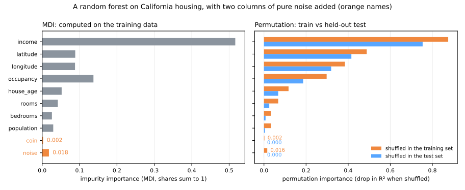
Held-out data, not training data
A forest with two noise columns: a continuous one and a coin flip.
Partial dependence: in which direction, with what shape?
Set feature \(j\) to a value \(v\) in every row, keep the rest, average the predictions (Friedman, 2001):
\[ \mathrm{PD}_j(v) = \frac{1}{n}\sum_{i=1}^{n} \hat f\bigl(x_{i,1}, \dots,\, v,\, \dots, x_{i,d}\bigr) \]\(n\): number of rows (4,087 test districts); \(x_{i,k}\): feature \(k\) of row \(i\), unchanged except feature \(j\), replaced by \(v\); \(\hat f\): the model's prediction.
by_hand = [model.predict(X_test.assign(income=v)).mean() for v in grid]
The PDP of income, by hand
Grid: income 1.5 to 10 ($10,000). Each step gives every one of the 4,087 rows that income. Predict. Does the predicted value grow steadily with income, or does it saturate?
ICE: one curve per row
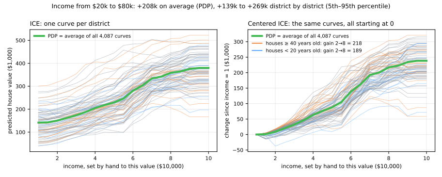
Income from $20,000 to $80,000: +$208,000 on average (the PDP), but from +$139,000 to +$269,000 district by district (5th to 95th percentile).
SHAP: why this prediction, for me?
Split one prediction into contributions, one per feature, that add up exactly:
\[ \hat f(x) = \underbrace{\phi_0}_{\text{base value}} + \phi_1 + \phi_2 + \dots + \phi_d \]- \(\phi_0\): the average prediction over a background dataset; \(\phi_j\): the share of feature \(j\) in the gap \(\hat f(x) - \phi_0\).
- Features are players; the prediction is the team's payout (Shapley, 1953; Lundberg & Lee, 2017).
- Value of a coalition \(S\), written \(v(S)\): set the features in \(S\) to the row's values, take the others from the background, average.
- \(\phi_j\): the average of \(v(S \cup \{j\}) - v(S)\) over the coalitions \(j\) can join, every order of arrival equally likely.
A toy model, small enough for a calculator
\[ f = 100 + 80\,\text{rich} + 60\,\text{coastal} + 40\,\text{rich}\cdot\text{coastal} + 20\,\text{big} \quad (\$1{,}000) \]- Background: four districts, worth 120, 180, 160 and 100. So \(v(\varnothing) = 140\).
- We explain a rich, coastal, not big district: \(f(x) = 280\).
Follow the arrows where "rich" joins
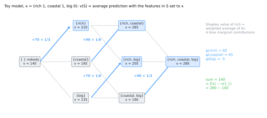
\(v(\{\text{rich}\})\): set rich = 1 in the four districts: 200, 180, 280, 180, average 210.
\[ \phi_{\text{rich}} = \tfrac13(210-140) + \tfrac16(285-195) + \tfrac16(205-135) + \tfrac13(280-190) = 80 \]Every number makes sense
rich: 80
main effect 80 × (1 − ¼) = 60, plus half of the interaction, 20
coastal: 65
45 + 20: the interaction is split equally
big: −5
20 × (0 − ¼): not big, while a quarter of the background is
80 + 65 − 5 = 140 = 280 − 140. The only attribution with these four properties:
efficiency (they add up) · symmetry · dummy (no effect → 0) · additivity (a sum of models → a sum of values)
shap.TreeExplainer on a tree that reproduces the formula returns [80, 65, −5] and base value 140.
Simulator: every coalition, every arrival order
Predict. Turn coastal off. Does the interaction still split in half? Does the waterfall still land on the prediction?
On the real model: a San Francisco district
- 8 features: \(2^8 = 256\) coalitions × 100 background districts = 25,600 predictions.
- Brute force and
TreeExplaineragree to the sixth decimal (largest difference 2e-06).
TreeExplainer gets the same exact numbers by walking each tree once per row (Lundberg et al., 2020).Reading a waterfall
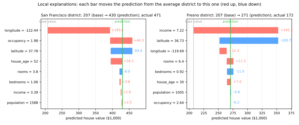
San Francisco (430k): longitude +185.6 and latitude −64.6, so location +121.0; low occupancy +66.3; old houses +34.2; an ordinary income, +2.6.
Fresno (271k): a high income (7.22) adds +145.2; location −88.3.
Global: local explanations, stacked
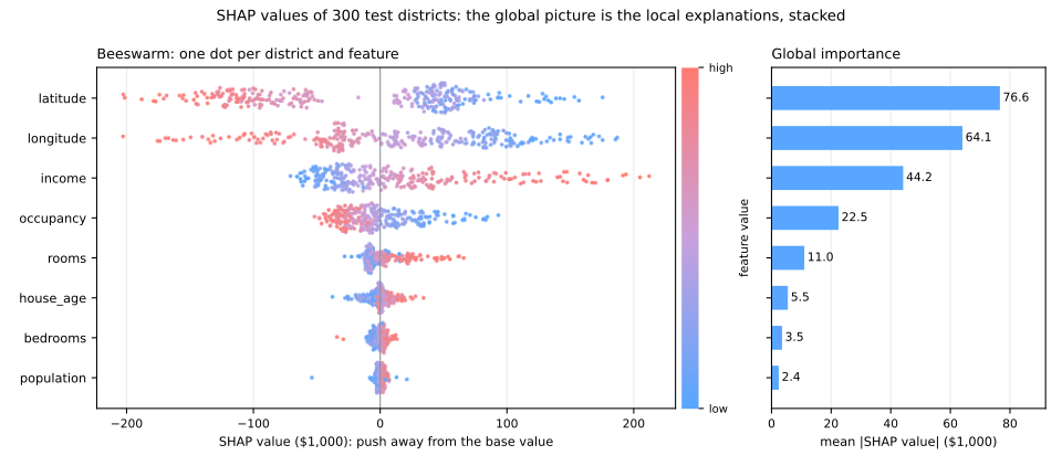
300 districts × 8 SHAP values. Mean |SHAP|, in $1,000: latitude 76.6, longitude 64.1, income 44.2, occupancy 22.5 ...
The beeswarm shows direction too: high incomes on the right, high occupancies and northern latitudes on the left.
Explanation ≠ causation
- "Low occupancy (1.98 people per household) adds $66,300 to the predicted price of the San Francisco district" (its SHAP value) is a true statement about the model.
- It does not mean that moving people out of a house makes it more expensive: crowded households are a marker of poorer neighborhoods.
- For auditing: if a credit model leans on the postcode, it may use it as a proxy for income or ethnicity.
Right for the wrong reasons
Hospital A: patients too sick to stand get the portable scanner. Hospital B: scanners assigned at random.
hospital B
permutation importance
scanner 0.393; medical markers 0.012 at most
markers only
73.0% on A, 74.7% on B
No validation on A could have warned you. The explanation did; only domain knowledge says the reliance will not survive.
Summary
- Readable first: if an interpretable model is as good on the same folds, use it.
- Permutation importance, on held-out data: how much the score needs each feature.
- PDP for the average shape of an effect, ICE for the rows behind it; fanning curves mean interactions.
- SHAP: contributions that add up exactly to prediction − base value; stacked, a global ranking with directions.
- An explanation describes the model, not the world; when one feature dominates, ask when is this value recorded?
| question | method |
|---|---|
| which features does the score need? | permutation importance, held-out |
| how does the prediction change with one feature? | PDP + ICE |
| why this prediction, for this row? | SHAP waterfall |
Explaining credit decisions, steps 1 to 7
- German credit: 1,000 loans, 20 attributes, 30% went bad.
- Scorecard or forest, on the same folds (ROC AUC, area under the receiver operating characteristic curve); then open the forest: MDI against permutation, PDP and ICE, SHAP globally and for the riskiest applicant.
- Download the lab notebook and open it in Jupyter or Colab (File → Upload notebook).
- At every step, answer the Predict before running.
- Simulations: permutation on the training rows (step 4) and a background of good loans only (step 7).
Pace: steps 1 to 3 in 10 min; step 4 and the first simulation in 10 min; steps 5 and 6 in 10 min; step 7 and the second simulation in 10 min.