Gradient Boosting
A random forest grows hundreds of deep trees independently and averages them: each tree overfits in its own way, and the average cancels the noise. Boosting does the opposite. It grows small trees, one after another, and each new tree is fitted to the errors the ensemble still makes. The forest fights variance; boosting fights bias. The idea started as a theoretical question (can many "weak" learners, each barely better than chance, be combined into a strong one?), became a practical algorithm with AdaBoost (Freund & Schapire, 1997), and was turned into a general recipe by Friedman (2001): gradient boosting, gradient descent where each step is a tree. Its engineered descendants, XGBoost (2016), LightGBM (2017) and CatBoost (2018), are still the default choice for tabular data in industry and competitions.
This lesson builds gradient boosting from a six-point example you can compute with a calculator, shows why the residuals are a gradient, measures each regularization knob, and ends with a lab on real bank-marketing data, where the modern libraries meet the random forest on the same folds. Every number quoted comes from the code blocks or from the figure scripts next to this page.
How this lesson is organized
The lesson has two approaches. Each has slides, text and a lab to do in class on Colab; the quiz at the end covers the fundamental one. Start with the fundamental approach: the advanced one builds on it.
| Fundamental approach | Advanced approach | |
|---|---|---|
| question | How does adding weak trees, one after another, make a strong model — and how do you stop it from overdoing it? | Which loss boosting optimizes, what the modern libraries change, and when it beats the forest |
| content | averaging against adding, boosting by hand on six points, residuals as a gradient, learning rate × number of trees, early stopping | other losses, classification on the log-odds, AdaBoost, the other knobs, histograms, XGBoost, LightGBM and CatBoost, forest or boosting |
| in-class lab | telemarketing: a leak, the default booster and the learning rate, steps 1 to 5 | forest, libraries, search, threshold and test, steps 6 to 11 |
| by the end, you can | run three rounds of boosting by hand; explain why more trees can hurt; use early stopping; spot a column that knows the future | choose the loss; read the Newton step of the leaves; compare libraries and the forest on the same folds; pick the threshold out-of-fold; distrust a random split on time-ordered data |
Both labs use the same notebook on Colab (in Portuguese): the fundamental part runs from step 1 to 5, the advanced part from step 6 to 11. Everything runs in the browser, including XGBoost and LightGBM, which come preinstalled on Colab; there is nothing to download.
Fundamental approach
One question drives this part: what happens when, instead of averaging independent trees, you add small trees, each fitted to what the previous ones got wrong? First with a calculator, on six points; then with the library. The algorithm is a gradient descent in which every step is a tree, and like every optimizer it does not know when to stop: the learning rate and early stopping are the brakes.
This part follows one path in four stages, drawn below: 1. add, do not average; 2. boost by hand; 3. residuals as a gradient; 4. brake and stop. Each stage links to its section, and in the slides a strip at the bottom shows which stage you are in.
- Add, do not averagesmall trees in sequence remove bias
- Boost by handfit the residuals, add them shrunk
- Residuals as a gradientgradient descent on the predictions
- Brake and stoplearning rate and early stopping
Fundamental approach slides
Click the slides and use the ← → arrows to navigate; F opens full screen and Esc shows every slide. Open the slides in a new tab
1. One small tree after another
Stage 1. The contrast with the forest is easiest to see on a problem where the right answer is known: a noisy sine curve, 200 training points, and 5,000 fresh points to measure the error. The noise alone has variance 0.25, so no model can have a test MSE below about 0.25.
import numpy as np
from sklearn.ensemble import GradientBoostingRegressor, RandomForestRegressor
from sklearn.tree import DecisionTreeRegressor


def sample(n, seed):                          # a noisy sine; the noise has variance 0.25
    r = np.random.default_rng(seed)
    X = r.uniform(0, 6, (n, 1))
    return X, 2 * np.sin(X[:, 0]) + r.normal(0, 0.5, n)


X, y = sample(200, seed=0)                    # training data
X_new, y_new = sample(5000, seed=1)           # fresh data, to measure the error

models = {
    'one stump':                DecisionTreeRegressor(max_depth=1),
    'forest of 200 stumps':     RandomForestRegressor(n_estimators=200, max_depth=1, random_state=0),
    'boosting of 200 stumps':   GradientBoostingRegressor(n_estimators=200, max_depth=1,
                                                          learning_rate=0.1, random_state=0),
    'one deep tree':            DecisionTreeRegressor(random_state=0),
    'forest of 200 deep trees': RandomForestRegressor(n_estimators=200, random_state=0),
}
for name, model in models.items():
    model.fit(X, y)
    train_mse = np.mean((model.predict(X) - y) ** 2)
    test_mse = np.mean((model.predict(X_new) - y_new) ** 2)
    print(f"{name:25s} training MSE {train_mse:.3f} · test MSE {test_mse:.3f}")
one stump                 training MSE 0.552 · test MSE 0.608
forest of 200 stumps      training MSE 0.511 · test MSE 0.572
boosting of 200 stumps    training MSE 0.215 · test MSE 0.280
one deep tree             training MSE 0.000 · test MSE 0.509
forest of 200 deep trees  training MSE 0.054 · test MSE 0.369
A stump is a tree with a single split: one question, two leaves. It is the classic weak learner: it can only say "left of the cut, this value; right of it, that value".
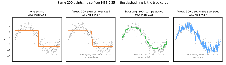
Read the table two rows at a time:
- Averaging does not remove bias. A forest of 200 stumps is barely better than one stump (test MSE 0.572 against 0.608). Every stump, whatever bootstrap sample it sees, makes roughly the same cut near the middle, so their average is still roughly one step. The error of a stump is bias: it is too simple to follow a sine, and 200 copies of "too simple" are still too simple.
- Averaging removes variance. A single deep tree memorizes the training set (training MSE 0.000) and pays for it on new data (0.509). Averaging 200 of them brings the test MSE down to 0.369. That is the forest's job, from the random forest lesson.
- Adding removes bias. Boosting uses the same weak stumps as the first forest, but it adds them: each new stump is fitted to what the previous ones got wrong. The result follows the curve and reaches a test MSE of 0.280, close to the noise floor of 0.25.
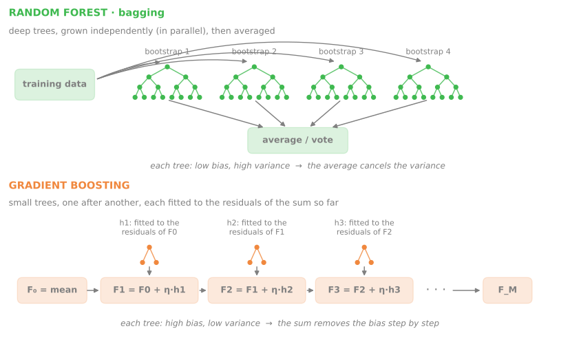
So the two ensembles are not rivals doing the same thing. A forest needs strong, unstable trees and averages them; boosting needs weak, stable trees and stacks them.
The diagram puts the two strategies side by side (figure script):
2. Boosting by hand
Six points, three stumps
Stage 2. Six points, one feature:
| \(x\) | 1 | 2 | 3 | 4 | 5 | 6 |
|---|---|---|---|---|---|---|
| \(y\) | 2 | 3 | 4 | 9 | 10 | 14 |
The loss is the squared error, and each round adds a stump multiplied by a learning rate \(\eta = 0.5\) (the same \(\eta\) as in gradient descent; why a half-step is a good idea comes later). The recipe:
- Start with a constant. The constant that minimizes the squared error is the mean: \(F_0 = 42/6 = 7\).
- Compute the residuals \(r_i = y_i - F_0(x_i)\): \(-5, -4, -3, 2, 3, 7\).
- Fit a stump to the residuals, not to \(y\). A stump on one feature tries every cut between neighboring points and keeps the one with the smallest squared error; each leaf predicts the mean residual of its points.
- Add it, shrunk: \(F_1 = F_0 + \eta \cdot \text{stump}_1\). Repeat from step 2.
Step 3, the stump search, is the regression tree of the decision trees lesson with depth 1:
x = np.arange(1, 7).reshape(-1, 1)
y = np.array([2, 3, 4, 9, 10, 14])

r = y - y.mean()                                   # residuals of F0 = 7
for t in [1.5, 2.5, 3.5, 4.5, 5.5]:                # the five possible cuts
    left, right = r[x.ravel() < t], r[x.ravel() > t]
    sse = ((left - left.mean()) ** 2).sum() + ((right - right.mean()) ** 2).sum()
    print(f"x < {t}: left mean {left.mean():+.2f} · right mean {right.mean():+.2f} · SSE {sse:.2f}")
x < 1.5: left mean -5.00 · right mean +1.00 · SSE 82.00
x < 2.5: left mean -4.50 · right mean +2.25 · SSE 51.25
x < 3.5: left mean -4.00 · right mean +4.00 · SSE 16.00
x < 4.5: left mean -2.50 · right mean +5.00 · SSE 37.00
x < 5.5: left mean -1.40 · right mean +7.00 · SSE 53.20
The cut at 3.5 wins by far (SSE 16, the next best is 37): the left leaf predicts \(-4\) and the right leaf \(+4\). With \(\eta = 0.5\), the ensemble moves half of the way: \(F_1 = 7 - 2 = 5\) for \(x \le 3\) and \(7 + 2 = 9\) for \(x \ge 4\). Now repeat with the new residuals:
| round | cut chosen | leaf values (left / right) | predictions \(F_m\) at \(x = 1 \dots 6\) | residuals | training MSE |
|---|---|---|---|---|---|
| 0 | — | — | 7, 7, 7, 7, 7, 7 | −5, −4, −3, 2, 3, 7 | 18.67 |
| 1 | \(x < 3.5\) | −4 / +4 | 5, 5, 5, 9, 9, 9 | −3, −2, −1, 0, 1, 5 | 6.67 |
| 2 | \(x < 5.5\) | −1 / +5 | 4.5, 4.5, 4.5, 8.5, 8.5, 11.5 | −2.5, −1.5, −0.5, 0.5, 1.5, 2.5 | 2.92 |
| 3 | \(x < 3.5\) | −1.5 / +1.5 | 3.75, 3.75, 3.75, 9.25, 9.25, 12.25 | −1.75, −0.75, 0.25, −0.25, 0.75, 1.75 | 1.23 |
Check round 2 with a calculator. The residuals after round 1 are \(-3, -2, -1, 0, 1, 5\); the big one left is the last point, so the best cut isolates it: \(x < 5.5\), left mean \((-3-2-1+0+1)/5 = -1\), right leaf \(5\). Half of that is added: \(5 - 0.5 = 4.5\), \(9 - 0.5 = 8.5\) and \(9 + 2.5 = 11.5\). Notice that round 3 uses the same cut as round 1: nothing forbids it, the residuals simply asked for more of the same correction.
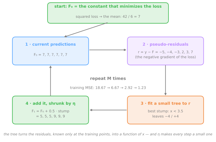
The whole loop fits in one diagram, with the numbers of the first round (figure script):
The library confirms
GradientBoostingRegressor with max_depth=1 builds stumps; staged_predict returns the predictions after each round:
gb = GradientBoostingRegressor(n_estimators=3, max_depth=1, learning_rate=0.5).fit(x, y)
for m, F in enumerate(gb.staged_predict(x), start=1):
    stump = gb.estimators_[m - 1, 0].tree_          # node 0 is the cut, nodes 1 and 2 the leaves
    print(f"round {m}: x < {stump.threshold[0]} · leaves {stump.value[1, 0, 0]:+.1f} / "
          f"{stump.value[2, 0, 0]:+.1f} · F = {F} · MSE {np.mean((y - F) ** 2):.2f}")
round 1: x < 3.5 · leaves -4.0 / +4.0 · F = [5. 5. 5. 9. 9. 9.] · MSE 6.67
round 2: x < 5.5 · leaves -1.0 / +5.0 · F = [ 4.5  4.5  4.5  8.5  8.5 11.5] · MSE 2.92
round 3: x < 3.5 · leaves -1.5 / +1.5 · F = [ 3.75  3.75  3.75  9.25  9.25 12.25] · MSE 1.23
Same cuts, same leaf values, same predictions. Note that the tree stores the unshrunk leaf values (\(-4\), \(+4\)); the learning rate is applied when the trees are added up.
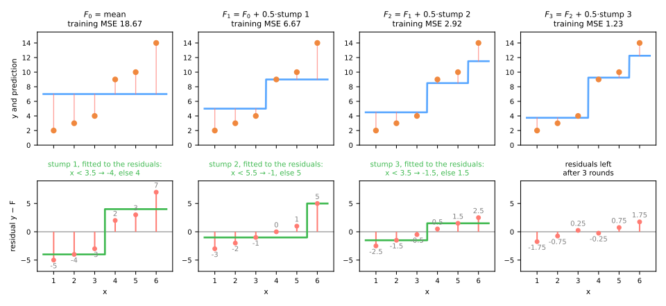
The top row is the ensemble after each round, a staircase that gets one more step (or a taller one) each time. The bottom row is what the next stump sees: not the data, but the residuals, which shrink round after round. The final model is a sum: \(F_3(x) = 7 + 0.5\,\text{stump}_1(x) + 0.5\,\text{stump}_2(x) + 0.5\,\text{stump}_3(x)\).
Watch the residual shrink
The simulator runs the same loop on 60 points. The bottom panel is the residual, and the green step function is the stump about to be fitted to it. The slider \(\nu\) is the learning rate (\(\nu\) is the letter Friedman used; scikit-learn calls it learning_rate, and this page calls it \(\eta\)).
Three experiments:
- Set ν = 1 with 6 stumps, then ν = 0.15 with 40. Both reach a similar fit, but the second got there in small, hedged steps. With \(\nu = 1\) each stump fully corrects its region, including the noise in it; with a small \(\nu\), a correction has to be confirmed by several consecutive stumps before it is fully applied.
- Halve \(\nu\) and you need roughly twice as many stumps for the same fit.
learning_rateandn_estimatorsare one knob seen from two sides, and must be tuned together. - Set ν = 1 and push the stumps to 60. The blue curve starts bending toward individual points while the training MSE keeps falling. The training error cannot tell you when to stop; a validation curve can, and below it turns back up.
3. Why "gradient" boosting: residuals are a gradient
Stage 3. Look at the squared loss of one point, as a function of the prediction \(F\):
The residual is the negative gradient of the loss with respect to the prediction. So the hand example did gradient descent, but not on weights: on the six predictions themselves. Round \(m\) computed the direction in which each prediction should move to lower the loss (the residuals), and moved each prediction a step \(\eta\) in that direction.
Why not move the six predictions directly, then? Because the gradient is only known at the training points, and the model must predict everywhere. Fitting a tree to the gradient turns six numbers into a function of \(x\): it groups points that want to move the same way, and gives every new \(x\) the step of its group. Friedman's general algorithm, for any differentiable loss \(L\):
F0(x) = the constant c that minimizes Σ L(yᵢ, c)            # the mean, the median, the log-odds...
for m = 1 .. M:
    rᵢ = −∂L(yᵢ, F)/∂F  at F = F_{m−1}(xᵢ)                  # pseudo-residuals: the negative gradient
    fit a small regression tree h_m to the pairs (xᵢ, rᵢ)     # the tree decides the regions
    in each leaf, set the value that lowers the loss most     # for squared error: the mean residual
    F_m(x) = F_{m−1}(x) + η · h_m(x)                           # a small step
The \(r_i\) are called pseudo-residuals: for the squared loss they are the ordinary residuals, for other losses they are something else, and the tree is always a regression tree fitted to them, even when the problem is classification.
4. The regularization toolkit: learning rate and early stopping
Stage 4. Boosting is an optimizer: every round lowers the training loss, and nothing in the algorithm stops it. On real data that means it eventually fits noise, so more trees can make the model worse, which never happens with a forest. The brakes, all used together:
- Learning rate \(\eta\): shrink each tree's contribution;
- Number of trees, chosen by early stopping on a validation set;
- Tree size:
max_depthormax_leaf_nodes; - Leaf size and penalties:
min_samples_leaf,l2_regularization; - Subsampling: each tree sees a random fraction of the rows (stochastic gradient boosting, Friedman 2002) and/or of the columns (
max_features,colsample_bytree), the forest's decorrelation trick.
This part measures the first two brakes, the ones that matter most; the others are left to section 9.
Learning rate and number of trees
The data for this section: California housing, 20,640 districts, predict the median house value (in thousands of dollars) from location, age, rooms, income and ocean proximity. Each model below adds 1,000 trees with no early stopping, and the validation error is recorded after every tree (figure script):
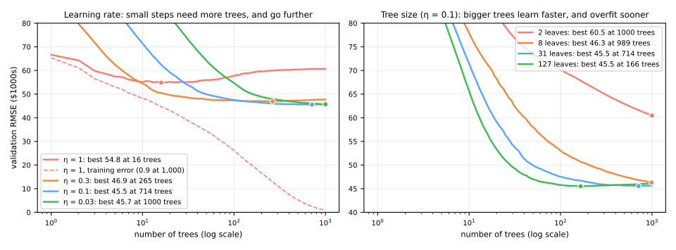
The left panel is the central picture of boosting:
- With \(\eta = 1\), the validation error bottoms out after 16 trees (54.8 thousand dollars) and then climbs to 60.7, while the training error (dashed) keeps falling, to 0.9 after 1,000 trees. That gap is overfitting, produced by adding trees.
- Smaller \(\eta\) takes more trees to get anywhere, but gets further: 46.9 at 265 trees for \(\eta = 0.3\), 45.5 at 714 for \(\eta = 0.1\). The curve after the minimum is also flatter, so overshooting the right number of trees costs less.
- Below some \(\eta\) the gains stop, and only the cost remains: after 1,000 trees \(\eta = 0.03\) is at 45.7 and still falling, while \(\eta = 0.1\) reached 45.5 at 714 trees.
The right panel changes the tree size at \(\eta = 0.1\). Stumps (2 leaves) cannot represent interactions between features, such as "close to the ocean and high income", and are still at 60.5 after 1,000 trees. Larger trees learn faster and reach their minimum sooner: 8 leaves reach 46.3 only at 989 trees, 31 leaves 45.5 at 714, 127 leaves 45.5 at 166, after which the error starts to creep back up. A tree with \(d\) levels can combine at most \(d\) features along a path, so the tree size caps the interaction order the model can express.
Early stopping picks the number of trees
Nobody draws that curve by hand in practice. Early stopping holds out a slice of the training data, watches the loss on it after every tree, and stops when it has not improved for n_iter_no_change rounds. The number of trees becomes an output, not a hyperparameter:
import pandas as pd
from sklearn.ensemble import HistGradientBoostingRegressor
from sklearn.model_selection import train_test_split

url = 'https://raw.githubusercontent.com/hsandmann/biblio/refs/heads/main/ml/aula02/housing.csv'
housing = pd.read_csv(url)
y_h = housing.pop('median_house_value') / 1000                   # in thousands of dollars
X_h = housing.astype({'ocean_proximity': 'category'})           # read natively, no encoding needed
X_tr, X_va, y_tr, y_va = train_test_split(X_h, y_h, test_size=0.25, random_state=0)

for eta in [1.0, 0.3, 0.1]:
    model = HistGradientBoostingRegressor(learning_rate=eta, max_iter=5000, early_stopping=True,
                                          validation_fraction=0.1, n_iter_no_change=20,
                                          random_state=0).fit(X_tr, y_tr)
    rmse = np.sqrt(np.mean((model.predict(X_va) - y_va) ** 2))
    print(f"η = {eta:<3}: stopped after {model.n_iter_:4d} trees · validation RMSE {rmse:.1f}")
η = 1.0: stopped after   41 trees · validation RMSE 56.4
η = 0.3: stopped after   87 trees · validation RMSE 47.4
η = 0.1: stopped after  337 trees · validation RMSE 46.0
Early stopping lands near the bottom of each curve of the figure without ever looking at X_va: 56.4 for \(\eta = 1\) (the figure's minimum was 54.8), 47.4 for \(\eta = 0.3\) and 46.0 for \(\eta = 0.1\). For \(\eta = 0.1\) it stopped at 337 trees, well before the figure's minimum at 714, because that curve is almost flat after 300 trees: 20 rounds without improvement on a small watch set are enough to call it, and the cost is half a point of RMSE. Two details to remember:
- the watch set is carved out of the training data (
validation_fraction=0.1), so the trees are fitted on 90% ofX_tr, and your own validation or test data stay untouched; - the fitted model keeps the
n_iter_no_changetrees added after the best one; scikit-learn does not roll back. With a large \(\eta\) those extra trees already overfit (the lab measures what that costs), with a small one they are harmless. Give small learning rates more patience.
5. Summary: boosting in five lines
- Averaging cuts variance; adding cuts bias. A forest of stumps is still roughly a stump; a boosting of stumps follows the curve.
- Each tree is fitted to the residuals of the current ensemble and enters multiplied by the learning rate \(\eta\): \(F_m = F_{m-1} + \eta\, h_m\).
- The residuals are the negative gradient of the loss: boosting is gradient descent on the predictions, with a tree turning the gradient into a function of \(x\).
- More trees can make the model worse. A smaller \(\eta\) needs more trees, goes further, and climbs more slowly past the minimum.
- Early stopping watches a slice of the training data and picks the number of trees by itself: it becomes an output, not a hyperparameter.
| symptom | what is happening | what to do |
|---|---|---|
| validation error lowest early, then rising | large \(\eta\): the following trees fit noise | lower \(\eta\) and switch on early stopping |
| error still falling at the end | too few trees for the chosen \(\eta\) | more trees (let early stopping decide) |
| perfect training, poor validation | overfitting by adding trees | early stopping, smaller trees, larger leaves |
| metrics too good to be true | a column that knows the future | ask, column by column, whether the value exists at prediction time |
Fundamental lab — who will subscribe?
The problem. A Portuguese bank ran phone campaigns between 2008 and 2010 to sell a term deposit (Moro, Cortez & Rita, 2014). Each of the 45,211 rows is one client contacted in a campaign: age, job, marital status, education, account balance, loans, how and when they were contacted, and what happened in previous campaigns. The target: did the client subscribe? Only 11.7% did. A model that ranks clients by their chance of subscribing lets the bank call the promising ones first.
The workflow is the one from the validation lesson: lock a test set away, one cv object for every model, compare on the same folds, touch the test set once, at step 10. The positive class is rare, so the headline metric is average precision (AP, the area under the precision–recall curve of the ROC and imbalanced data lesson), with ROC AUC alongside. This part finds a leak, measures the default booster against a linear model, and tunes the learning rate with early stopping; the forest, the other libraries, the search, the threshold and the test are left to the advanced lab.
How to do this lab in class (about 35 min, in pairs)
- Open the lab notebook on Colab (in Portuguese). There is nothing to download or install: Colab runs in the browser and already has XGBoost and LightGBM. To keep your answers, save a copy to your Drive (File → Save a copy in Drive) before editing. Run the cells in order, in a single session.
- This lab is steps 1 to 5 of the notebook. The advanced lab continues in the same notebook, from step 6.
- Every step starts with a Predict: answer it with your partner before running the cell. Getting the prediction wrong is what makes the result memorable.
- After running, compare with the output and the reading on this page. Every output here is exactly what the code prints.
- The Simulations ask you to write a small Python experiment: change one input and watch what happens to the output. No hand calculations. The solution is collapsed right below: try before opening it.
- Suggested pace: steps 1 to 3 in 10 min; step 4 and the first simulation in 12 min; step 5 and the second simulation in 13 min. Steps 4 and 5 take from a few seconds to a minute to run.
Step 1 — load, name the columns, look
Predict. Only part of the clients contacted subscribe to the deposit. Do you expect something close to 50%, 25% or 10%? And the call duration: longer for those who subscribed or for those who did not?
import numpy as np
import pandas as pd
from sklearn.datasets import fetch_openml

bank = fetch_openml(data_id=1461, as_frame=True)            # Bank Marketing (UCI), one row per client
X = bank.data.copy()
X.columns = ['age', 'job', 'marital', 'education', 'default', 'balance', 'housing', 'loan',
             'contact', 'day', 'month', 'duration', 'campaign', 'pdays', 'previous', 'poutcome']
y = (bank.target == '2').astype(int).rename('subscribed')   # 1 = subscribed a term deposit
print(X.shape, f"· subscribed: {y.sum()} ({y.mean():.1%})")
print(X.dtypes.astype(str).value_counts().to_dict())
print(X['duration'].describe().round(0).to_dict())
print(X.groupby(y)['duration'].median())
(45211, 16) · subscribed: 5289 (11.7%)
{'category': 9, 'int64': 7}
{'count': 45211.0, 'mean': 258.0, 'std': 258.0, 'min': 0.0, '25%': 103.0, '50%': 180.0, '75%': 319.0, 'max': 4918.0}
subscribed
0    164.0
1    426.0
Name: duration, dtype: float64
45,211 clients, of whom 5,289 (11.7%) subscribed. Nine columns are categorical (pandas category, which boosting can use directly) and seven are integers. OpenML ships the columns anonymized as V1…V16; the names above follow the order of the original UCI documentation, and it is worth checking at least one against the data before trusting the list. Column 12, duration, is documented as the duration of the last call, in seconds: its values run from 0 to 4,918 (82 minutes) with a median of 180 (three minutes), which is what phone calls look like. And it separates the classes strongly: clients who subscribed talked for a median of 426 seconds, the others for 164.
Step 2 — lock the test set away, fix the folds, set a baseline
Predict. With 11.7% positives, what AP does a random ordering of the clients get? And what ROC AUC?
from sklearn.dummy import DummyClassifier
from sklearn.model_selection import StratifiedKFold, cross_validate, train_test_split

X_dev, X_test, y_dev, y_test = train_test_split(X, y, test_size=0.2, stratify=y, random_state=42)
cv = StratifiedKFold(n_splits=5, shuffle=True, random_state=42)     # the SAME folds for every model


def cv_eval(model, X_=None):
    """5-fold CV on the development set: fold scores, fit times and the fitted fold models."""
    return cross_validate(model, X_dev if X_ is None else X_, y_dev, cv=cv, return_estimator=True,
                          scoring=['roc_auc', 'average_precision'])


def summary(r):
    return (f"ROC AUC {r['test_roc_auc'].mean():.3f} ± {r['test_roc_auc'].std():.3f} · "
            f"AP {r['test_average_precision'].mean():.3f} ± {r['test_average_precision'].std():.3f}")


print(X_dev.shape, X_test.shape)
print('dummy', summary(cv_eval(DummyClassifier(strategy='prior'))))
36,168 rows for development and 9,043 locked away until step 10, both with 11.7% positives thanks to stratify=y. The cv object is created once and every model below is scored on the same five folds, so differences can be compared fold by fold. The dummy's AP is 0.117, the prevalence: that is what a random ranking scores, and every AP below must be read against it, not against 0 or 0.5. Its ROC AUC is 0.5, the ROC baseline.
Step 3 — a leak in plain sight: the call duration
Predict. The call duration separates subscribers from the rest very well. Can it be used to decide whom to call? What do you expect from the metrics without it?
from sklearn.ensemble import HistGradientBoostingClassifier

hgb = HistGradientBoostingClassifier(random_state=42)
with_duration = cv_eval(hgb)
without = cv_eval(hgb, X_dev.drop(columns='duration'))
print('with duration   ', summary(with_duration))
print('without duration', summary(without))

X_dev, X_test = X_dev.drop(columns='duration'), X_test.drop(columns='duration')   # gone for good
with duration    ROC AUC 0.934 ± 0.002 · AP 0.624 ± 0.017
without duration ROC AUC 0.797 ± 0.004 · AP 0.447 ± 0.012
With duration, the booster reaches ROC AUC 0.934 and AP 0.624. Without it, 0.797 and 0.447. The most useful column in the table is also unusable: the length of a call is known only when the call is over, and the model's job is to decide whom to call. The UCI documentation says so itself (the column "should be discarded if the intention is to have a realistic predictive model"). This is the leak of features that know the future: no cross-validation scheme can detect it, because it lives in the columns, not in the split. The question has to be asked of every column: is this value available at the moment the prediction is made? From here on, duration is gone from both X_dev and X_test, and 0.797 is the honest starting point.
Step 4 — HistGradientBoosting out of the box, against a linear model
Predict. The booster uses the columns as they are, with no one-hot and no scaling; the logistic regression gets everything prepared. Which one ranks the clients better?
from sklearn.compose import make_column_selector, make_column_transformer
from sklearn.linear_model import LogisticRegression
from sklearn.pipeline import make_pipeline
from sklearn.preprocessing import OneHotEncoder, OrdinalEncoder, StandardScaler

categorical = make_column_selector(dtype_include='category')
logistic = make_pipeline(
    make_column_transformer((OneHotEncoder(handle_unknown='ignore'), categorical),
                            remainder=StandardScaler()),
    LogisticRegression(max_iter=2000))
as_codes = make_pipeline(
    make_column_transformer((OrdinalEncoder(), categorical), remainder='passthrough'),
    HistGradientBoostingClassifier(categorical_features=None, random_state=42))

results = {'logistic regression': cv_eval(logistic),
           'HGB, native categories': without,
           'HGB, categories as codes': cv_eval(as_codes)}
for name, r in results.items():
    print(f"{name:25s}", summary(r))
print('trees kept by early stopping in each fold:', [m.n_iter_ for m in without['estimator']])
logistic regression       ROC AUC 0.763 ± 0.003 · AP 0.402 ± 0.008
HGB, native categories    ROC AUC 0.797 ± 0.004 · AP 0.447 ± 0.012
HGB, categories as codes  ROC AUC 0.795 ± 0.002 · AP 0.441 ± 0.010
trees kept by early stopping in each fold: [52, 45, 46, 59, 71]
How to read it:
- Boosting against a linear model. The logistic regression, with one-hot encoded categories and scaled numbers, reaches ROC AUC 0.763 and AP 0.402. The booster, with no preprocessing at all, reaches 0.797 and 0.447: 4.5 points of AP, about four fold standard deviations. The trees find thresholds and interactions between columns that a linear model cannot represent without hand-made features.
- Native categories against integer codes. Feeding the categories natively (0.447) or as arbitrary integer codes (0.441) makes a difference smaller than the fold standard deviation here. With codes, the trees must cut an arbitrary order (
admin.= 0,blue-collar= 1, …) into pieces, which costs more splits; with 12 jobs and 12 months the trees manage anyway. The native route matters more with many categories, and it is simpler: no encoder to fit. - Early stopping was already on.
HistGradientBoostingClassifierswitches it on by itself when there are more than 10,000 rows (early_stopping='auto'), with at mostmax_iter=100trees. Each fold kept between 45 and 71.
Simulation: a forest of stumps against a boosting of stumps. Section 1 compared, on a sine, the average of 200 stumps with the sum of 200 stumps. Repeat it on the bank data, on the same folds: a single stump, a forest of 200 stumps and a boosting of 200 stumps (max_leaf_nodes=2, no early stopping). How much of the gap to the full booster does each one close?
Solution
from sklearn.ensemble import RandomForestClassifier

codes = lambda: make_column_transformer((OrdinalEncoder(), categorical), remainder='passthrough')
stumps = {'one stump': make_pipeline(codes(), RandomForestClassifier(
              n_estimators=1, max_depth=1, bootstrap=False, max_features=None, random_state=42)),
          'forest of 200 stumps': make_pipeline(codes(), RandomForestClassifier(
              n_estimators=200, max_depth=1, n_jobs=-1, random_state=42)),
          'boosting of 200 stumps': HistGradientBoostingClassifier(
              max_leaf_nodes=2, max_iter=200, early_stopping=False, random_state=42)}    # stump = 2 leaves
for name, model in stumps.items():
    print(f"{name:23s}", summary(cv_eval(model)))
one stump               ROC AUC 0.546 ± 0.003 · AP 0.153 ± 0.003
forest of 200 stumps    ROC AUC 0.720 ± 0.004 · AP 0.283 ± 0.010
boosting of 200 stumps  ROC AUC 0.775 ± 0.003 · AP 0.412 ± 0.007
A single stump barely ranks anything (AP 0.153, close to the 0.117 prevalence). The forest of stumps improves a lot (0.283), unlike the sine of section 1: here there are 15 columns and the forest's feature draw makes each stump cut a different column, so the average becomes a rough sum of effects from several columns. But each stump was fitted without knowing about the others. Boosting fits each stump to what the previous ones still get wrong and reaches 0.412, close to the default booster's 0.447, using only one-question trees. What is missing to get there are the interactions between columns, which a stump cannot represent.
Step 5 — learning rate × number of trees, with early stopping
Predict. With \(\eta = 0.5\), will the booster need more or fewer trees than with \(\eta = 0.03\)? And will it go further or less far?
import matplotlib.pyplot as plt

for eta in [0.5, 0.1, 0.03]:
    model = HistGradientBoostingClassifier(learning_rate=eta, max_iter=2000, early_stopping=True,
                                           n_iter_no_change=30, random_state=42)
    results[f'HGB, η = {eta}'] = r = cv_eval(model)
    trees = [m.n_iter_ for m in r['estimator']]
    print(f"η = {eta:<4} trees per fold {trees} · {summary(r)}")
    curve = -r['estimator'][0].validation_score_          # fold 0: log loss on its inner 10%
    plt.plot(curve, label=f'η = {eta}')
plt.xscale('log'); plt.xlabel('trees'); plt.ylabel('inner validation log loss'); plt.legend()
plt.show()
η = 0.5  trees per fold [38, 36, 34, 36, 35] · ROC AUC 0.768 ± 0.008 · AP 0.385 ± 0.008
η = 0.1  trees per fold [99, 108, 80, 79, 105] · ROC AUC 0.795 ± 0.002 · AP 0.446 ± 0.014
η = 0.03 trees per fold [349, 296, 206, 304, 270] · ROC AUC 0.798 ± 0.004 · AP 0.449 ± 0.015
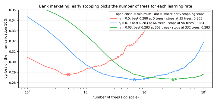
(figure script, fitted on the whole development set rather than on one fold)
How to read it:
- η = 0.5 is clearly worse: ROC AUC 0.768 and AP 0.385, against 0.795 and 0.446 for η = 0.1. The figure shows why. The inner validation loss is lowest after only 5 trees, then climbs; early stopping needs 30 rounds without improvement before it stops, and the model keeps those 30 overfitting trees (loss 0.305 at the stop, against 0.288 at the minimum).
- η = 0.1 and η = 0.03 tie: AP 0.446 and 0.449, a difference far smaller than the fold standard deviations (0.014–0.015). With small steps the valley is wide and flat, so the 30 extra trees cost almost nothing (0.284 against 0.283). The smaller rate needs about three times as many trees (206–349 against 79–108) for no measurable gain.
- The number of trees is an output. Nobody chose 99, 108, 80, 79 or 105: the folds did.
Simulation: more trees, no brakes. Switch early stopping off and fix the number of trees at 5, 35, 200 and 1,000, with \(\eta = 0.5\) and \(\eta = 0.05\). To be quick, use only the first fold of cv and measure the AP on its validation part. Do more trees always help?
Solution
from sklearn.metrics import average_precision_score

tr, va = next(cv.split(X_dev, y_dev))                  # a single fold, to be quick
print('trees   η = 0.5   η = 0.05')
for n in [5, 35, 200, 1000]:
    aps = []
    for eta in [0.5, 0.05]:
        m = HistGradientBoostingClassifier(learning_rate=eta, max_iter=n, early_stopping=False, random_state=42)
        m.fit(X_dev.iloc[tr], y_dev.iloc[tr])
        aps.append(average_precision_score(y_dev.iloc[va], m.predict_proba(X_dev.iloc[va])[:, 1]))
    print(f"{n:5d}   {aps[0]:7.3f}   {aps[1]:8.3f}")
With \(\eta = 0.5\), the AP peaks after just 5 trees (0.418) and falls with every batch of trees, down to 0.336 with 1,000: the following trees fit noise. With \(\eta = 0.05\) the climb is slower and the peak higher (0.435 with 200 trees), but the fall comes all the same: 0.408 with 1,000. In a forest more trees never hurt; in boosting they do, and the right point depends on \(\eta\). That is exactly the job early stopping did by itself in step 5, fold by fold.
To close the fundamental part. In one sentence each: (1) why does adding stumps fitted to the residuals go further than averaging stumps? (2) Why can the call duration not enter the model, however much it improves the metrics? (3) What does early stopping decide, and with which data?
Your turn (fundamental)
At home:
- One more round by hand. Continue the six-point example of section 2: compute the residuals after round 3, find the best split and the leaves of the fourth stump, and the predictions \(F_4\). Check with
GradientBoostingRegressor(n_estimators=4, max_depth=1, learning_rate=0.5). - Put the leak back. Rerun steps 4 and 5 keeping
durationinX_dev. How much does the AP rise? Write one paragraph for the bank's manager explaining why that model cannot go to production, and another suggesting howdurationcould be used (hint: once the call has started, to decide whether to keep talking). - Stumps with early stopping. Fit
HistGradientBoostingClassifier(max_leaf_nodes=2, max_iter=5000, early_stopping=True, n_iter_no_change=30)on the same folds. How many trees does early stopping keep? Does the AP reach the default booster's 0.447?
Advanced approach
The fundamental part built boosting with the squared loss and braked it with the learning rate. This part shows what changes when the loss changes and what the libraries do for you: robust losses, classification on the log-odds with Newton steps, AdaBoost as a special case, the other knobs, the engineering tricks of XGBoost, LightGBM and CatBoost, and a fair comparison with the forest. The code blocks continue those of sections 1 to 4.
This part follows one path in four stages, drawn below: 1. any loss, same loop; 2. tune the other knobs; 3. the modern libraries; 4. forest or boosting? Each stage links to its section, and in the slides a strip at the bottom shows which stage you are in.
- Any loss, same looprobust losses, log-odds, AdaBoost
- Tune the other knobstree size, leaves, L2, with η fixed
- The modern librarieshistograms, XGBoost, LightGBM, CatBoost
- Forest or boosting?a fair comparison, side by side
Advanced approach slides
Click the slides and use the ← → arrows to navigate; F opens full screen and Esc shows every slide. Open the slides in a new tab
6. Other losses, same machinery
| loss | \(L(y, F)\) | pseudo-residual \(-\partial L / \partial F\) | \(F_0\) |
|---|---|---|---|
| squared error | \(\tfrac12 (y - F)^2\) | \(y - F\) | mean |
| absolute error | \(\lvert y - F \rvert\) | \(\operatorname{sign}(y - F)\) | median |
| Huber | squared near 0, absolute beyond \(\delta\) | \(y - F\), clipped to \(\pm\delta\) | — |
| log loss (classification) | \(-[y \ln p + (1-y)\ln(1-p)]\), \(p = \sigma(F)\) | \(y - p\) | log-odds of the base rate |
Stage 1. The loss decides what the next tree listens to. Make the last point of the example an outlier, \(y_6 = 40\) instead of 14:
y_out = np.array([2, 3, 4, 9, 10, 40])
F0_sq, F0_abs = y_out.mean(), np.median(y_out)
print(f"squared loss : F0 = {F0_sq:.2f} (mean)   pseudo-residuals {np.round(y_out - F0_sq, 2)}")
print(f"absolute loss: F0 = {F0_abs:.2f} (median) pseudo-residuals {np.sign(y_out - F0_abs)}")
squared loss : F0 = 11.33 (mean)   pseudo-residuals [-9.33 -8.33 -7.33 -2.33 -1.33 28.67]
absolute loss: F0 = 6.50 (median) pseudo-residuals [-1. -1. -1.  1.  1.  1.]
Under the squared loss the outlier's pseudo-residual (28.67) is three times larger than any other, so the first stump will spend its cut on that single point. Under the absolute loss every point pushes with the same strength, \(\pm 1\): the outlier says "higher" exactly as loudly as the 9 and the 10 do. That is why loss='absolute_error' or loss='huber' is the choice when the target has heavy tails; loss='quantile' fits a quantile instead of the mean, which gives prediction intervals. Changing the loss changes one line of the algorithm.
7. Classification: boosting the log-odds
For a 0/1 target the ensemble does not add up probabilities (a sum of trees could leave \([0, 1]\)). It adds up log-odds, exactly the quantity \(F\) of logistic regression, and turns the sum into a probability with the sigmoid, \(p = 1/(1 + e^{-F})\). The pseudo-residual of the log loss is \(y - p\): how far the current probability is from the label.
Six points again, the label now 0 or 1:
| \(x\) | 1 | 2 | 3 | 4 | 5 | 6 |
|---|---|---|---|---|---|---|
| \(y\) | 0 | 1 | 0 | 1 | 1 | 1 |
By hand, one round with \(\eta = 0.5\).
- \(F_0\) is the log-odds of the base rate: 4 positives out of 6, \(p = 2/3\), \(F_0 = \ln\frac{2/3}{1/3} = \ln 2 = 0.693\).
- Pseudo-residuals \(y - p\): \(-0.667, 0.333, -0.667, 0.333, 0.333, 0.333\).
- The stump search on these numbers picks the cut \(x < 3.5\) (SSE 0.667, against 0.8 for the next best).
- The leaf values are not the mean pseudo-residual here. scikit-learn takes one Newton step in each leaf: the sum of the gradients divided by the sum of the second derivatives, \(\sum (y_i - p_i) / \sum p_i (1 - p_i)\). Left leaf: \((-0.667 + 0.333 - 0.667) / (3 \times \tfrac{2}{9}) = -1/\tfrac{2}{3} = -1.5\). Right leaf: \(+1/\tfrac{2}{3} = +1.5\).
- \(F_1 = 0.693 - 0.5 \times 1.5 = -0.057\) on the left and \(0.693 + 0.75 = 1.443\) on the right. Through the sigmoid: \(p = 0.486\) and \(p = 0.809\).
from sklearn.ensemble import GradientBoostingClassifier

yc = np.array([0, 1, 0, 1, 1, 1])
p0 = yc.mean()
F0 = np.log(p0 / (1 - p0))                               # log-odds of the base rate
g = yc - p0                                              # pseudo-residuals y - p
left = x.ravel() < 3.5
newton = lambda m: g[m].sum() / (p0 * (1 - p0) * m.sum())  # one Newton step per leaf
F1 = F0 + 0.5 * np.where(left, newton(left), newton(~left))
p1 = 1 / (1 + np.exp(-F1))
log_loss = lambda p: -np.mean(yc * np.log(p) + (1 - yc) * np.log(1 - p))
print(f"F0 = {F0:.3f} · leaves {newton(left):+.2f} / {newton(~left):+.2f}")
print(f"by hand     : F1 = {F1.round(3)} · p1 = {p1.round(3)}")

clf = GradientBoostingClassifier(n_estimators=1, max_depth=1, learning_rate=0.5).fit(x, yc)
print(f"scikit-learn: F1 = {clf.decision_function(x).round(3)} · p1 = {clf.predict_proba(x)[:, 1].round(3)}")
print(f"log loss: {log_loss(np.full(6, p0)):.3f} before, {log_loss(p1):.3f} after one round")
F0 = 0.693 · leaves -1.50 / +1.50
by hand     : F1 = [-0.057 -0.057 -0.057  1.443  1.443  1.443] · p1 = [0.486 0.486 0.486 0.809 0.809 0.809]
scikit-learn: F1 = [-0.057 -0.057 -0.057  1.443  1.443  1.443] · p1 = [0.486 0.486 0.486 0.809 0.809 0.809]
log loss: 0.637 before, 0.448 after one round
The library agrees to the third decimal, and one stump lowers the log loss from 0.637 to 0.448. The Newton step divides by \(p(1-p)\), the curvature of the log loss: where the model is still unsure (\(p\) near 0.5) the curvature is largest and the step is cautious, where it is already confident the step can be bigger. Keep this formula in mind: XGBoost uses it for every loss, and adds a penalty to it, below.
8. AdaBoost, the ancestor
Gradient boosting was not the first boosting algorithm. AdaBoost (Freund & Schapire, 1997) answered the weak-learner question with a different mechanism: instead of fitting residuals, it reweights the training points. Each round trains a stump on the weighted data, then raises the weights of the points it got wrong and lowers the others, so the next stump is forced to look at the hard cases. With labels \(\pm 1\) and a stump of weighted error \(\varepsilon\):
The final classifier is the sign of the weighted vote \(\sum_m \alpha_m h_m(x)\): a stump with small error gets a large \(\alpha\). Ten points, equal weights, a stump that gets three of them wrong:
w = np.full(10, 0.1)
wrong = np.array([0, 0, 1, 0, 0, 1, 0, 0, 1, 0], dtype=bool)   # 3 misclassified points
eps = w[wrong].sum()
alpha = 0.5 * np.log((1 - eps) / eps)
w = w * np.exp(np.where(wrong, alpha, -alpha))
w = w / w.sum()
print(f"error {eps:.1f} · vote alpha {alpha:.3f}")
print(f"new weight of a misclassified point {w[wrong][0]:.4f}, of a correct one {w[~wrong][0]:.4f}")
print(f"total weight on the misclassified points: {w[wrong].sum():.2f}")
error 0.3 · vote alpha 0.424
new weight of a misclassified point 0.1667, of a correct one 0.0714
total weight on the misclassified points: 0.50
The three hard points went from 10% to 16.7% of the weight each, and together they now hold exactly half of it. That is not a coincidence of these numbers: after the update the previous stump always has a weighted error of exactly 50%, the level of a coin flip, so the next stump cannot simply repeat it and must find something new. Friedman, Hastie & Tibshirani (2000) later showed that AdaBoost is gradient boosting in disguise, with the exponential loss \(e^{-yF}\); gradient boosting generalized it to any loss, which is why it replaced AdaBoost in practice.
Does stacking weak learners really make a strong one? The classic test (Hastie, Tibshirani & Friedman, The Elements of Statistical Learning, §10.1): 10 Gaussian features, the label is \(+1\) when their sum of squares exceeds 9.34, 2,000 training points and 10,000 test points.
from sklearn.datasets import make_hastie_10_2
from sklearn.ensemble import AdaBoostClassifier
from sklearn.tree import DecisionTreeClassifier

Xh, yh = make_hastie_10_2(n_samples=12000, random_state=1)
Xh_tr, yh_tr, Xh_te, yh_te = Xh[:2000], yh[:2000], Xh[2000:], yh[2000:]
contenders = {
    'one stump':                    DecisionTreeClassifier(max_depth=1),
    'one deep tree':                DecisionTreeClassifier(random_state=0),
    'AdaBoost, 400 stumps':         AdaBoostClassifier(DecisionTreeClassifier(max_depth=1),
                                                       n_estimators=400, random_state=0),
    'gradient boosting, 400 stumps': GradientBoostingClassifier(n_estimators=400, max_depth=1,
                                                                random_state=0),
}
for name, model in contenders.items():
    err = 1 - model.fit(Xh_tr, yh_tr).score(Xh_te, yh_te)
    print(f"{name:30s} test error {err:.1%}")
one stump                      test error 45.9%
one deep tree                  test error 24.5%
AdaBoost, 400 stumps           test error 11.6%
gradient boosting, 400 stumps  test error 11.1%
A stump is almost a coin flip here (45.9% error): no single cut on one feature says much about a sum of ten squares. A fully grown tree gets 24.5%. Four hundred stumps, each as weak as the first, get 11.6% (AdaBoost) and 11.1% (gradient boosting): the weak learners, combined, beat the strong one by more than half.
9. The other knobs, one at a time
Stage 2. With \(\eta = 0.1\) and early stopping fixed, change one knob at a time and measure it with 5-fold cross-validation (the cross-validation lesson), always on the same folds:
from sklearn.model_selection import KFold, cross_validate

cv_h = KFold(n_splits=5, shuffle=True, random_state=0)
base = dict(learning_rate=0.1, max_iter=5000, early_stopping=True, n_iter_no_change=20, random_state=0)
variants = {'defaults (31 leaves)': {},
            'max_leaf_nodes=8': {'max_leaf_nodes': 8},
            'max_leaf_nodes=127': {'max_leaf_nodes': 127},
            'min_samples_leaf=200': {'min_samples_leaf': 200},
            'l2_regularization=10': {'l2_regularization': 10},
            'max_features=0.5': {'max_features': 0.5}}
for name, extra in variants.items():
    r = cross_validate(HistGradientBoostingRegressor(**base, **extra), X_h, y_h, cv=cv_h,
                       scoring='neg_root_mean_squared_error', return_estimator=True)
    trees = np.mean([m.n_iter_ for m in r['estimator']])
    print(f"{name:21s} RMSE {-r['test_score'].mean():.1f} ± {r['test_score'].std():.1f} · {trees:4.0f} trees")
defaults (31 leaves)  RMSE 45.8 ± 0.6 ·  350 trees
max_leaf_nodes=8      RMSE 46.3 ± 0.8 ·  736 trees
max_leaf_nodes=127    RMSE 45.9 ± 0.6 ·  179 trees
min_samples_leaf=200  RMSE 46.4 ± 0.3 ·  452 trees
l2_regularization=10  RMSE 45.5 ± 0.4 ·  419 trees
max_features=0.5      RMSE 45.8 ± 0.7 ·  343 trees
Once the learning rate and the number of trees are right, the other knobs barely matter on this data: every variant lands between 45.5 and 46.4, at most 0.6 away from the defaults, which is the size of the defaults' own fold standard deviation (0.6). The paired comparison of the cross-validation lesson would be needed before calling any of them better. What the knobs do change is how many trees are needed: 8-leaf trees need 736 on average, 127-leaf trees 179. Tree size and number of trees trade against each other, like the learning rate and the number of trees. On smaller or noisier data, where overfitting comes sooner, min_samples_leaf, the L2 penalty and subsampling earn their keep; that is why they belong in the search, not in a fixed recipe.
HistGradientBoosting* has no row subsampling; XGBoost and LightGBM do (subsample, which LightGBM applies only when subsample_freq > 0), and a simulation of the advanced lab (step 7) measures it.
A tuning order that works
- Fix a moderate learning rate (0.05–0.1) and turn on early stopping, so the number of trees takes care of itself. 2. Tune the tree size (
max_leaf_nodes/max_depth/num_leaves) and the leaf size, with cross-validation. 3. Try row and column subsampling and the L2 penalty. 4. For the final model, lower the learning rate (and let early stopping add trees) if the extra training time is affordable. The random and Bayesian searches of the AutoML lesson do steps 2–3 more efficiently than a grid.
10. The modern libraries
Stage 3. Friedman's algorithm, as in GradientBoostingRegressor, sorts every feature at every split. The libraries that made boosting the default for tabular data keep the algorithm and change the engineering.
Histograms (LightGBM, XGBoost tree_method='hist', scikit-learn's HistGradientBoosting*). Before training, each feature is cut into at most 255 bins by its quantiles, and every split search runs over bin boundaries instead of sorted values. The cost of a split no longer grows with the number of distinct values, only with the number of bins, and the loss in precision is negligible. The binning also gives two things for free: missing values get their own bin, and at each split the tree learns whether they go left or right; and categorical features can be split into groups of categories directly, with no one-hot encoding (categorical_features='from_dtype' reads the pandas category dtype, as in the code above).
XGBoost (Chen & Guestrin, 2016) adds a penalty to each tree and uses the second derivative of the loss for every step. For a tree with \(T\) leaves and leaf values \(w_j\), the objective of one round is
and a second-order expansion of the loss gives the best value of each leaf in closed form, with \(G_j\) and \(H_j\) the sums of first and second derivatives over the leaf:
With \(\lambda = 0\) this is exactly the Newton step computed by hand for the classification example: left leaf \(G = \sum (p - y) = 1\), \(H = \sum p(1-p) = 0.667\), \(w^* = -1.5\). With reg_lambda=1 (XGBoost's default), \(w^* = -1/1.667 = -0.6\): the penalty pulls small, poorly supported leaves toward zero, the Ridge idea applied inside the tree. \(\gamma\) charges for each extra leaf, so a split is kept only if it lowers the loss by more than \(\gamma\).
LightGBM (Ke et al., 2017) grows trees leaf-wise: instead of splitting every node of one level before going to the next, it always splits the leaf whose split lowers the loss most, anywhere in the tree. For the same number of leaves this fits more, so its main size knob is num_leaves, not max_depth (scikit-learn's HistGradientBoosting* grows leaf-wise too, with max_leaf_nodes). Two further tricks make it fast on large data: GOSS keeps all the rows with large gradients and samples the rest, and EFB bundles sparse features that are never non-zero together into one.
CatBoost (Prokhorenkova et al., 2018) specializes in categorical features: it encodes each category by the mean target of the rows seen before it in a random order (so a row never sees its own label, a built-in guard against target leakage), and it grows symmetric trees, where every node of a level uses the same split.
The same knobs, under four names:
| idea | scikit-learn HistGradientBoosting* | XGBoost | LightGBM | CatBoost |
|---|---|---|---|---|
| learning rate | learning_rate | learning_rate (eta) | learning_rate | learning_rate |
| number of trees | max_iter | n_estimators | n_estimators | iterations |
| tree size | max_leaf_nodes, max_depth | max_depth, max_leaves | num_leaves, max_depth | depth |
| leaf size | min_samples_leaf | min_child_weight (in second-derivative units) | min_child_samples | min_data_in_leaf |
| L2 penalty on leaves | l2_regularization | reg_lambda | reg_lambda | l2_leaf_reg |
| row subsampling | — | subsample | subsample (bagging_fraction) | subsample |
| column subsampling | max_features (per split) | colsample_bytree | colsample_bytree | rsm |
| early stopping | early_stopping=True | early_stopping_rounds + eval_set | callbacks=[lgb.early_stopping(...)] | early_stopping_rounds |
The lab compares the scikit-learn, XGBoost and LightGBM implementations on the same folds, for accuracy and for time.
11. Forest or boosting?
Stage 4. Both are ensembles of trees, both need no scaling, both handle interactions and nonlinearity. Which one? Three measurements on California housing, all on the same 5 folds.
Out of the box. Default settings, fold by fold:
from sklearn.ensemble import RandomForestRegressor

X_codes = X_h.assign(ocean_proximity=X_h['ocean_proximity'].cat.codes)   # the forest needs numbers
contenders = {'random forest, defaults': (RandomForestRegressor(n_jobs=-1, random_state=0), X_codes),
              'boosting, defaults': (HistGradientBoostingRegressor(random_state=0), X_h),
              'boosting, tuned': (HistGradientBoostingRegressor(
                  learning_rate=0.05, max_iter=5000, max_leaf_nodes=63, early_stopping=True,
                  n_iter_no_change=30, random_state=0), X_h)}
rmse, fit_time = {}, {}
for name, (model, data) in contenders.items():
    r = cross_validate(model, data, y_h, cv=cv_h, scoring='neg_root_mean_squared_error')
    rmse[name], fit_time[name] = -r['test_score'], r['fit_time'].mean()
    print(f"{name:24s} RMSE per fold {rmse[name].round(1)} → {rmse[name].mean():.1f}")
for other in ['boosting, defaults', 'boosting, tuned']:
    d = rmse['random forest, defaults'] - rmse[other]
    print(f"forest − {other:18s}: {d.round(1)} → {d.mean():+.1f} ± {d.std():.1f}")
random forest, defaults  RMSE per fold [49.7 48.6 48.7 49.2 49.3] → 49.1
boosting, defaults       RMSE per fold [47.4 47.3 47.4 47.8 47.9] → 47.5
boosting, tuned          RMSE per fold [45.6 45.  44.4 45.9 45.8] → 45.3
forest − boosting, defaults: [2.3 1.4 1.4 1.4 1.4] → +1.6 ± 0.4
forest − boosting, tuned   : [4.2 3.6 4.3 3.3 3.5] → +3.8 ± 0.4
With defaults, boosting beats the forest in every fold, by 1.4 to 2.3 thousand dollars of RMSE (mean +1.6 ± 0.4). The "tuned" booster is not the result of a search: it is the knob experiment above read out loud, a smaller learning rate (0.05) with early stopping and larger trees (63 leaves). It reaches 45.3 and beats the forest in every fold by 3.3 to 4.3 (mean +3.8 ± 0.4). By the rule of the cross-validation lesson, both differences are far larger than the spread of the paired differences: real. The same caveat as always: this configuration was picked after looking at experiments on the same folds, so its 45.3 is slightly optimistic.
Tuning sensitivity. Draw 16 random configurations of each family and score them all on the same folds, with R² as the score (figure script). Forest: max_features from 0.2 to 1.0 and min_samples_leaf from 1 to 20, 100 trees. Boosting: learning rate from 0.01 to 1, 50 to 1,000 trees without early stopping, 4 to 127 leaves, 5 to 100 rows per leaf.
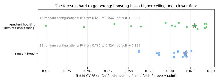
The forest's 16 configurations all land between R² 0.762 and 0.826, and its defaults (0.819) sit near the top: almost whatever you pick, you get a decent forest. Boosting's configurations spread three times wider, from 0.650 to 0.844. Its best configurations beat every forest, and even its defaults (0.830) beat all 16 of them. Its worst are not exotic, just mismatched: the three lowest points all combine a small learning rate (0.02 to 0.05) with only 50 or 100 trees, and stop long before the curves of the learning-rate figure reach their bottom; at the other extreme, a learning rate near 0.7 or 1 run for 100 to 1,000 trees also ends below the forest's defaults. The best one, 0.047 with 1,000 trees of 16 leaves, sits in between. This is why boosting is tuned with early stopping: it takes the most dangerous knob, the number of trees, out of the search.
Time. The fit times of the first block, on the machine that built this page:
Seconds depend on the machine, so your output will differ. The machine that built this page was busy with other jobs, so these numbers were measured with every model restricted to one CPU core (n_jobs=1 for the forest, OMP_NUM_THREADS=1 for the booster), which keeps the comparison fair:
random forest, defaults  11.5 s per fit
boosting, defaults       0.5 s per fit
boosting, tuned          2.7 s per fit
On one core, the forest takes 11.5 s per fit and the default booster 0.5 s, more than twenty times less: the forest grows 100 fully grown trees on bootstrap samples of the 16,512 training rows, the booster at most 100 small trees on 255-bin histograms. Even the tuned booster, with larger trees, a smaller learning rate and a few hundred trees, takes 2.7 s. Both parallelize on more cores: the forest across trees, the histogram booster inside each tree.
| Random forest | Gradient boosting | |
|---|---|---|
| trees are built | independently, in parallel | one after another, each correcting the rest |
| each tree is | deep, unstable (low bias, high variance) | shallow, stable (high bias, low variance) |
| the ensemble reduces | variance, by averaging | bias, by adding |
| more trees | never hurt, only cost time | eventually overfit: use early stopping |
| out of the box | very good, hard to break | good; bad settings can be much worse |
| tuned | a little better | usually the best on tabular data |
| key knobs | max_features, min_samples_leaf | learning_rate + number of trees, tree size |
| free extras | out-of-bag error, parallel training | early stopping, native missing values and categories, custom losses |
When each wins. Reach for a forest when you want a strong baseline with almost no tuning, when the data is small and noisy, or when you need an honest error estimate for free (out-of-bag). Reach for boosting when the last points of accuracy matter and you can afford cross-validated tuning, when the data is large (histogram implementations are fast), or when the loss is unusual (quantiles, ranking, Poisson counts). On tabular data, tuned gradient boosting still routinely beats deep learning (Grinsztajn et al., 2022); for images, audio and text, neural networks take over.
12. Practical profile
| Gradient boosting (histogram libraries) | |
|---|---|
| Data | tabular: numeric and categorical columns, missing values allowed |
| Preprocessing | none required: no scaling, no imputation, no one-hot encoding (categories as category dtype) |
| Tasks | regression (squared, absolute, Huber, quantile, Poisson…), binary and multiclass classification, ranking |
| Key hyperparameters | learning rate and number of trees (via early stopping), tree size, leaf size, subsampling, L2 |
| Training cost | sequential in the trees, parallel inside each tree; histogram versions handle millions of rows |
| Prediction cost | one pass down each tree: fast |
| Failure modes | overfits with too many trees at a high learning rate; extrapolates as a constant outside the training range (like every tree model); probabilities can need calibration |
| Interpretability | not readable tree by tree; use permutation importance (in the lab) or SHAP values, which have an exact, fast algorithm for tree ensembles (Explainability) |
Advanced lab — compare, tune and test
The fundamental lab ended with an honest booster (no duration), where a learning rate of 0.1 with early stopping tied with 0.03 at a third of the cost. This part compares it with the forest and with XGBoost and LightGBM on the same folds, tunes a few knobs, picks a threshold on out-of-fold predictions, opens the test set once, and asks which columns the model leans on. Continue in the same notebook, in the same session: the steps below use X_dev, y_dev, cv, cv_eval, summary, categorical and results from steps 1 to 5.
How to do this lab in class (about 40 min, in pairs)
- Continue in the Colab notebook, from step 6. If the session dropped, first run the cells of steps 1 to 5 (Runtime → Run before).
- As in the fundamental lab: Predict before running, compare with this page, and try the Simulations before opening the solution.
- Suggested pace: steps 6 and 7 and the first simulation in 15 min (the forest takes half a minute); step 8 in 10 min (the search takes a minute or two); steps 9 and 10 in 8 min; step 11 and the second simulation in 7 min.
Step 6 — the random forest, on the same folds
Predict. The forest averages deep trees; boosting adds small ones. On these data, will the gap between the two be large or small?
from sklearn.ensemble import RandomForestClassifier

forest = make_pipeline(
    make_column_transformer((OrdinalEncoder(), categorical), remainder='passthrough'),
    RandomForestClassifier(n_estimators=300, min_samples_leaf=5, n_jobs=-1, random_state=42))
results['random forest'] = cv_eval(forest)
print('random forest', summary(results['random forest']))

a, b = results['HGB, η = 0.1'], results['random forest']
for metric in ['roc_auc', 'average_precision']:
    d = a['test_' + metric] - b['test_' + metric]
    print(f"HGB − forest, {metric:17s}: {d.round(3)} → {d.mean():+.3f} ± {d.std():.3f}")
random forest ROC AUC 0.790 ± 0.004 · AP 0.439 ± 0.015
HGB − forest, roc_auc          : [-0.001  0.006  0.005  0.005  0.011] → +0.005 ± 0.004
HGB − forest, average_precision: [0.006 0.01  0.005 0.011 0.004] → +0.007 ± 0.003
The forest needs numbers, so its categories go through an OrdinalEncoder (trees only need an order to cut, not one-hot columns). min_samples_leaf=5 is a common choice for a noisy target; tuning it is part of Your turn. The forest reaches ROC AUC 0.790 and AP 0.439, close behind the booster, and the paired differences settle it: boosting is ahead in all five folds on AP (+0.007 ± 0.003) and in four of five on ROC AUC (+0.005 ± 0.004). By the rule of the cross-validation lesson the AP difference is real, because it is more than twice the spread of the differences. It is also small: less than one point of AP. On this data the forest, with almost no tuning, gets nearly everything the booster gets.
Step 7 — XGBoost and LightGBM, same folds
Predict. XGBoost, LightGBM and scikit-learn's boosting implement the same algorithm. Will any of them stand out in AP? And in time?
import lightgbm as lgb
import xgboost as xgb

results['XGBoost'] = cv_eval(xgb.XGBClassifier(
    n_estimators=300, learning_rate=0.05, max_depth=5, tree_method='hist',
    enable_categorical=True, n_jobs=-1, random_state=42, verbosity=0))
results['LightGBM'] = cv_eval(lgb.LGBMClassifier(
    n_estimators=300, learning_rate=0.05, num_leaves=31, n_jobs=-1, random_state=42, verbose=-1))
for name in ['HGB, η = 0.1', 'random forest', 'XGBoost', 'LightGBM']:
    print(f"{name:14s}", summary(results[name]))
HGB, η = 0.1   ROC AUC 0.795 ± 0.002 · AP 0.446 ± 0.014
random forest  ROC AUC 0.790 ± 0.004 · AP 0.439 ± 0.015
XGBoost        ROC AUC 0.798 ± 0.002 · AP 0.452 ± 0.013
LightGBM       ROC AUC 0.798 ± 0.004 · AP 0.447 ± 0.011
The three boosting libraries tie: AP 0.446 (scikit-learn), 0.452 (XGBoost) and 0.447 (LightGBM), differences of at most 0.006 against fold standard deviations of 0.011–0.015, and ROC AUC 0.795–0.798. They implement the same algorithm; what differs is the engineering around it. The settings are not identical either (a fixed 300 trees at η = 0.05 for XGBoost and LightGBM, early stopping for scikit-learn), and a difference of this size would reverse with a different seed. All three are ahead of the forest (AP 0.439).
times = pd.DataFrame({name: {'fit (s)': r['fit_time'].mean(), 'predict (s)': r['score_time'].mean()}
                      for name, r in results.items()}).T
print(times.round(2))
Times depend on the machine, so this output will differ on yours. The machine that built this page was busy with other jobs, so these numbers were measured with every library restricted to one CPU core (n_jobs=1 for the forest, XGBoost and LightGBM, OMP_NUM_THREADS=1 for scikit-learn's boosting), which keeps the comparison fair:
                          fit (s)  predict (s)
logistic regression          0.06         0.01
HGB, native categories       0.30         0.03
HGB, categories as codes     0.35         0.03
HGB, η = 0.5                 0.33         0.05
HGB, η = 0.1                 0.60         0.04
HGB, η = 0.03                1.52         0.12
random forest                9.67         0.45
XGBoost                      0.88         0.07
LightGBM                     0.77         0.18
On one core, the three boosters fit a fold in under a second (0.60 s for scikit-learn at η = 0.1, 0.88 s for XGBoost, 0.77 s for LightGBM), the forest of 300 deep trees in 9.67 s, more than ten times longer. The smaller learning rate costs what the previous step promised: η = 0.03 takes 1.52 s for its roughly three times more trees. The forest is also the slowest to predict (0.45 s, against 0.04–0.18 s for the boosters), because every prediction walks down 300 deep trees. With several cores (the code uses n_jobs=-1) all of these shrink. On 29,000 rows every booster is fast; the speed tricks of LightGBM and XGBoost matter on millions of rows, which this lab does not have.
Simulation: stochastic boosting. Stochastic gradient boosting (Friedman, 2002) draws a fraction of the rows for every tree, and XGBoost also draws the columns, the forest's decorrelation trick. Add subsample=0.8 and colsample_bytree=0.8 to the XGBoost of step 7 and compare with it fold by fold. Is the difference larger than the spread of the paired differences?
Solution
sub = cv_eval(xgb.XGBClassifier(
    n_estimators=300, learning_rate=0.05, max_depth=5, tree_method='hist', subsample=0.8,
    colsample_bytree=0.8, enable_categorical=True, n_jobs=-1, random_state=42, verbosity=0))
print('XGBoost            ', summary(results['XGBoost']))
print('XGBoost, subsample ', summary(sub))
d = sub['test_average_precision'] - results['XGBoost']['test_average_precision']
print(f"difference in AP per fold: {d.round(3)} → {d.mean():+.3f} ± {d.std():.3f}")
XGBoost             ROC AUC 0.798 ± 0.002 · AP 0.452 ± 0.013
XGBoost, subsample  ROC AUC 0.801 ± 0.002 · AP 0.454 ± 0.012
difference in AP per fold: [ 0.005  0.003 -0.002  0.     0.001] → +0.001 ± 0.002
Subsampling raises the AP by 0.001 on average, with one fold going the other way and another tied: +0.001 ± 0.002 is a tie by the rule of the cross-validation lesson. ROC AUC goes from 0.798 to 0.801, also within the noise. With about 29,000 training rows per fold and small trees, the booster has little variance left to cut; subsampling usually matters more on smaller or noisier data — and, as a bonus, it makes every tree cheaper.
Step 8 — tune a few knobs with a random search
Predict. Ten random configurations, each with early stopping: will the gain over the step-5 model be larger or smaller than the gain from removing the leak, or from swapping the logistic regression for boosting?
from scipy.stats import loguniform, randint
from sklearn.model_selection import RandomizedSearchCV

space = {'learning_rate': loguniform(0.02, 0.3),
         'max_leaf_nodes': randint(8, 64),
         'min_samples_leaf': randint(10, 200),
         'l2_regularization': loguniform(1e-3, 10),
         'max_features': [0.5, 0.8, 1.0]}
search = RandomizedSearchCV(
    HistGradientBoostingClassifier(max_iter=2000, early_stopping=True, n_iter_no_change=30,
                                   random_state=42),
    space, n_iter=10, cv=cv, scoring='average_precision', random_state=42)
search.fit(X_dev, y_dev)
res = pd.DataFrame(search.cv_results_).sort_values('rank_test_score')
print(res[['param_learning_rate', 'param_max_leaf_nodes', 'param_min_samples_leaf',
           'mean_test_score', 'std_test_score']].head(4).round(3).to_string(index=False))
print(f"best AP {search.best_score_:.3f} (HGB, η = 0.1: "
      f"{results['HGB, η = 0.1']['test_average_precision'].mean():.3f})")
 param_learning_rate  param_max_leaf_nodes  param_min_samples_leaf  mean_test_score  std_test_score
               0.046                    51                      98            0.453           0.016
               0.029                    29                      62            0.451           0.014
               0.068                    11                      98            0.451           0.013
               0.067                    18                      97            0.451           0.015
best AP 0.453 (HGB, η = 0.1: 0.446)
Ten random configurations, each with early stopping, all scored on the same folds. The best (learning rate 0.046, 51 leaves, at least 98 rows per leaf) reaches AP 0.453, against 0.446 for the η = 0.1 model of step 5. The top four configurations are within 0.002 of each other and each has a fold standard deviation of 0.013–0.016, so the search found a plateau, not a peak, and its winner is the best of ten noisy estimates (the winner's curse of the cross-validation lesson). Compare the gains: removing the leak changed AP by 0.18, moving from a linear model to boosting by 0.045, tuning by 0.007. Tuning is worth doing, but after the data questions, not instead of them. For larger searches, random search is the right tool and Bayesian optimization (Optuna) is better; both are in the AutoML lesson.
Step 9 — choose the threshold on out-of-fold predictions
Predict. With 11.7% positives, will the threshold that maximizes F1 sit above or below 0.5? What share of the clients would the bank end up calling?
from sklearn.metrics import precision_recall_curve
from sklearn.model_selection import cross_val_predict

best = search.best_estimator_                   # refit on all of X_dev by the search
oof = cross_val_predict(best, X_dev, y_dev, cv=cv, method='predict_proba')[:, 1]
precision, recall, thresholds = precision_recall_curve(y_dev, oof)
f1 = 2 * precision * recall / (precision + recall + 1e-12)
k = f1[:-1].argmax()
threshold = thresholds[k]
print(f"threshold {threshold:.3f} · out-of-fold precision {precision[k]:.3f} · "
      f"recall {recall[k]:.3f} · F1 {f1[k]:.3f}")
print(f"share of clients flagged: {(oof >= threshold).mean():.1%}")
threshold 0.218 · out-of-fold precision 0.457 · recall 0.526 · F1 0.489
share of clients flagged: 13.5%
cross_val_predict gives every development row a probability from a model that did not train on it, so the threshold can be chosen on honest predictions without touching the test set (the ROC and imbalanced data lesson chose it on a validation split; these are 36,168 predictions instead). Maximizing F1 gives a threshold of 0.218, well below 0.5, as expected with 11.7% positives. At that threshold the bank would call 13.5% of its clients; 45.7% of those calls would be subscribers (against 11.7% calling at random, about four times better), and they would reach 52.6% of all subscribers. F1 weighs precision and recall equally; with the real cost of a call and the value of a deposit, the bank would choose the threshold that maximizes profit instead, with the same curve.
Step 10 — the one and only test
Predict. Will the test AP land close to the 0.453 of cross-validation? And precision and recall, close to the out-of-fold estimates of step 9?
from sklearn.metrics import average_precision_score, confusion_matrix, roc_auc_score

proba = best.predict_proba(X_test)[:, 1]
pred = (proba >= threshold).astype(int)
print(f"test ROC AUC {roc_auc_score(y_test, proba):.3f} · AP {average_precision_score(y_test, proba):.3f}")
print(confusion_matrix(y_test, pred, labels=[1, 0]))
tp, fn, fp, tn = confusion_matrix(y_test, pred, labels=[1, 0]).ravel()
print(f"precision {tp / (tp + fp):.3f} · recall {tp / (tp + fn):.3f}")
Once, at the end, the tuned booster meets the 9,043 test clients: ROC AUC 0.804, AP 0.465, slightly above the cross-validated 0.453 and within one fold standard deviation of it. At the threshold chosen in step 9, the model flags 1,209 clients (641 + 568, 13.4%): 568 of them subscribe, a precision of 0.470, and they are 53.7% of the 1,058 subscribers in the test set. Both numbers match the out-of-fold estimates of step 9 (0.457 and 0.526), which is what a leak-free pipeline looks like. The 490 subscribers the model misses are the price of calling only 13% of the list.
Step 11 — which columns does the model use?
Predict. Which columns do you expect the model to lean on most to predict who subscribes? Could any of them describe the moment of the campaign rather than the client?
from sklearn.inspection import permutation_importance

imp = permutation_importance(best, X_test, y_test, scoring='average_precision',
                             n_repeats=5, random_state=42)
print(pd.Series(imp.importances_mean, index=X_test.columns).sort_values(ascending=False).head(6).round(3))
Permutation importance shuffles one column at a time on the test set and measures how much the AP drops: a column the model relies on hurts when shuffled. The month of the contact (0.139) and the outcome of the previous campaign (0.132) dominate, followed by the contact channel and the day of the month. Read the top one critically. According to the UCI documentation the rows are ordered in time, from May 2008 to November 2010, and a random split mixes those periods. A model that leans on the month may be learning when the bank happened to call successfully, a pattern that need not hold next year; only a chronological split (TimeSeriesSplit, the cross-validation lesson) can tell. Tree ensembles are not readable one tree at a time; permutation importance gives a global view, and SHAP values, which have an exact and fast algorithm for tree ensembles, explain individual predictions (Explainability).
Simulation: and the following year? The rows are in time order (May 2008 to November 2010), but the lab split them at random. Simulate real use: train the winning configuration of step 8 on the first 80% of the rows and test on the last 20%; compare with the random test of step 10. Read the AP together with each test set's share of positives.
Solution
from sklearn.metrics import average_precision_score, roc_auc_score

Xt = X.drop(columns='duration')
cut = int(0.8 * len(Xt))                               # the rows are in time order
splits = {'random 80/20 (as in the lab)': (X_dev.index, X_test.index),
          'chronological: first 80% → last 20%': (Xt.index[:cut], Xt.index[cut:])}
for name, (a, b) in splits.items():
    m = HistGradientBoostingClassifier(max_iter=2000, early_stopping=True, n_iter_no_change=30,
                                       random_state=42, **search.best_params_)
    m.fit(Xt.loc[a], y.loc[a])
    p = m.predict_proba(Xt.loc[b])[:, 1]
    print(f"{name:37s} test positives {y.loc[b].mean():.1%} · ROC AUC {roc_auc_score(y.loc[b], p):.3f}"
          f" · AP {average_precision_score(y.loc[b], p):.3f}")
random 80/20 (as in the lab)          test positives 11.7% · ROC AUC 0.804 · AP 0.465
chronological: first 80% → last 20%   test positives 31.6% · ROC AUC 0.685 · AP 0.494
On the chronological test the ROC AUC drops from 0.804 to 0.685: the model ranks the clients of the next period much worse than those of the same period, shuffled together. The AP goes up (0.494), but only because the last period has 31.6% subscribers, almost three times as many; relative to prevalence it falls from 4.0 times a random list (0.465 / 0.117) to 1.6 times (0.494 / 0.316). The month and the outcome of the previous campaign, the two most important columns of step 11, describe a bank that changed over time. The random split answered "how well does the model interpolate within this period?"; the bank's question is "how well does it predict the next one?", and only the chronological split answers it.
To close the lesson. In one sentence each: (1) why do the three boosting libraries tie on AP but not on time? (2) Why can the threshold be chosen on out-of-fold predictions, without spending the test set? (3) What did the chronological split reveal that the random split hid?
Your turn (advanced)
At home, with more time:
- Early stopping inside XGBoost and LightGBM. Hold out 10% of
X_dev(stratified) as an evaluation set and fitxgb.XGBClassifier(n_estimators=3000, learning_rate=0.03, early_stopping_rounds=50, ...)witheval_set=[(X_eval, y_eval)]; do the same with LightGBM, usingcallbacks=[lgb.early_stopping(50)]. How many trees does each one keep? Compare with then_iter_of step 5. - A tuned forest. Tune the forest's
max_featuresandmin_samples_leafwith aRandomizedSearchCVof the same size as step 8, on the samecv. Does it close the gap to the tuned booster? Then read the AutoML lesson and redo step 8 with Optuna and 50 trials: how much of the gain had the 10 random trials already captured? - Validation in time. Redo the step-4 comparison (logistic regression against the booster) with
TimeSeriesSplit(n_splits=5)over the rows in their original order, withoutduration. Does the booster still win? By how much, and with what spread across folds?
References
- Schapire, R. E. "The Strength of Weak Learnability." Machine Learning 5 (1990): 197–227 — the first proof that weak learners can be boosted. DOI
- Freund, Y.; Schapire, R. E. "A Decision-Theoretic Generalization of On-Line Learning and an Application to Boosting." Journal of Computer and System Sciences 55, no. 1 (1997): 119–139 — AdaBoost. DOI
- Friedman, J. H.; Hastie, T.; Tibshirani, R. "Additive Logistic Regression: A Statistical View of Boosting." Annals of Statistics 28, no. 2 (2000): 337–407 — AdaBoost as stagewise fitting of the exponential loss. DOI
- Friedman, J. H. "Greedy Function Approximation: A Gradient Boosting Machine." Annals of Statistics 29, no. 5 (2001): 1189–1232 — gradient boosting, shrinkage, pseudo-residuals. DOI
- Friedman, J. H. "Stochastic Gradient Boosting." Computational Statistics & Data Analysis 38, no. 4 (2002): 367–378 — row subsampling. DOI
- Chen, T.; Guestrin, C. "XGBoost: A Scalable Tree Boosting System." KDD (2016): 785–794. DOI
- Ke, G.; Meng, Q.; Finley, T.; Wang, T.; Chen, W.; Ma, W.; Ye, Q.; Liu, T.-Y. "LightGBM: A Highly Efficient Gradient Boosting Decision Tree." Advances in Neural Information Processing Systems 30 (2017). Link
- Prokhorenkova, L.; Gusev, G.; Vorobev, A.; Dorogush, A. V.; Gulin, A. "CatBoost: Unbiased Boosting with Categorical Features." Advances in Neural Information Processing Systems 31 (2018). arXiv
- Hastie, T.; Tibshirani, R.; Friedman, J. The Elements of Statistical Learning, 2nd ed. Springer (2009), chapter 10 — boosting and additive trees; the 10-feature test problem. DOI
- Grinsztajn, L.; Oyallon, E.; Varoquaux, G. "Why Do Tree-Based Models Still Outperform Deep Learning on Typical Tabular Data?" NeurIPS Datasets and Benchmarks (2022). arXiv
- Pace, R. K.; Barry, R. "Sparse Spatial Autoregressions." Statistics & Probability Letters 33, no. 3 (1997): 291–297 — the California housing data. DOI
- Moro, S.; Cortez, P.; Rita, P. "A Data-Driven Approach to Predict the Success of Bank Telemarketing." Decision Support Systems 62 (2014): 22–31 — the lab's dataset (OpenML 1461). DOI
- XGBoost / LightGBM — gradient boosting.
Quiz
The quiz covers the fundamental approach.