Machine Learning · Insper

Gradient Boosting

Advanced approach

Other losses, the modern libraries, and when boosting beats the forest

The path of this part

Any loss, same looprobust losses, log-odds, AdaBoost
Tune the other knobstree size, leaves, L2, with η fixed
The modern librarieshistograms, XGBoost, LightGBM, CatBoost
Forest or boosting?a fair comparison, side by side

Each stage answers one question: what does the next tree listen to? → which knobs matter once the learning rate and early stopping are set? → what do the libraries add to the algorithm? → which ensemble should I use?

Stage 1 · what does the next tree listen to?

The loss decides what the next tree listens to

loss	pseudo-residual \(-\partial L/\partial F\)	\(F_0\)
squared	\(y - F\)	mean
absolute	\(\operatorname{sign}(y - F)\)	median
Huber	\(y - F\), clipped at \(\pm\delta\)	—
log loss	\(y - p\)	log-odds of the base rate

An outlier, \(y_6 = 40\): squared pseudo-residuals −9.33 … 28.67; absolute ones, all \(\pm 1\).

With the squared loss, the first stump spends its split on the outlier; with the absolute or Huber loss, every point pushes equally hard.

Classification: adding log-odds

The ensemble adds \(F\) (log-odds) and applies the sigmoid: \(p = 1/(1 + e^{-F})\). Pseudo-residual: \(y - p\).
Six points, 4 positive: \(F_0 = \ln 2 = 0.693\). The stump splits at \(x < 3.5\).
Each leaf gets a Newton step: \(\sum (y_i - p_i) / \sum p_i (1 - p_i) = \pm 1.5\).

\[ F_1 = 0.693 \pm 0.5 \times 1.5 \;\Rightarrow\; p = 0.486 \text{ and } 0.809 \]

By hand and scikit-learn agree to three decimals; one stump lowers the log loss from 0.637 to 0.448. Dividing by \(p(1-p)\), the curvature, keeps the step cautious where the model is unsure.

AdaBoost, the ancestor

Instead of residuals, it reweights the points: the misclassified gain weight, so the next stump must look at them.
A stump wrong on 3 of 10: \(\alpha = \tfrac12 \ln\frac{0.7}{0.3} = 0.424\); each misclassified point goes from 10% to 16.7%; together, half the weight.

10 features, sum of squares (ESL §10.1)	test error
one stump	45.9%
one full tree	24.5%
AdaBoost, 400 stumps	11.6%
gradient boosting, 400 stumps	11.1%

Stage 2 · which knobs matter once the learning rate and early stopping are set?

The other knobs, with \(\eta\) and early stopping fixed

California housing, 5-fold CV	RMSE	trees
defaults (31 leaves)	45.8 ± 0.6	350
`max_leaf_nodes=8`	46.3 ± 0.8	736
`max_leaf_nodes=127`	45.9 ± 0.6	179
`min_samples_leaf=200`	46.4 ± 0.3	452
`l2_regularization=10`	45.5 ± 0.4	419

Once \(\eta\) and the number of trees are right, the other knobs change the error little and how many trees are needed a lot. Tuning order: moderate \(\eta\) + early stopping → tree and leaf size → subsampling and L2.

Stage 3 · what do the libraries add to the algorithm?

The modern libraries

Histograms (LightGBM, XGBoost hist, HistGradientBoosting*): up to 255 bins per feature; native missing values and categories.
XGBoost: a penalty per tree and the second derivative; each leaf's optimal value is

\[ w_j^* = -\frac{G_j}{H_j + \lambda} \qquad \lambda = 0:\ -1.5 \quad \lambda = 1:\ -0.6 \]

LightGBM: grows leaf-wise (num_leaves), GOSS and EFB for large data.
CatBoost: encodes categories by the target mean of earlier rows, never seeing the row's own label.

With \(\lambda = 0\), \(w^*\) is the Newton step done by hand; \(\lambda\) is Ridge inside each leaf.

Stage 4 · which ensemble should I use?

Forest or boosting?

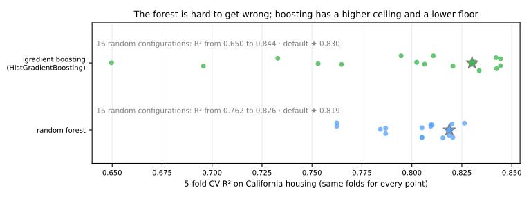
R² of 16 random forest and boosting configurations

Defaults, fold by fold: boosting beats the forest on every fold, +1.6 ± 0.4 thousand of RMSE; tuned, +3.8 ± 0.4.
16 random configurations: forest from R² 0.762 to 0.826; boosting from 0.650 to 0.844.

The forest is hard to spoil; tuned boosting goes further, but a mismatched configuration ends up much worse. Early stopping takes the most dangerous knob out of the search.

Side by side

	Random forest	Gradient boosting
trees	independent, deep	in sequence, shallow
reduces	variance (average)	bias (sum)
more trees	never hurt	end up overfitting
untuned	very good	good; bad settings can be much worse
tuned	a little better	usually the best on tabular data
for free	OOB, parallel training	early stopping, missing values, losses

Advanced lab · about 40 min, in pairs

Compare, tune and test, steps 6 to 11

Same notebook, same session: the steps use X_dev, cv, cv_eval, summary and results.
The forest, XGBoost and LightGBM on the same folds; a random search; the out-of-fold threshold; the test, once; the columns the model uses.
Notebook on Colab (in Portuguese), from step 6.
Simulations: stochastic boosting (step 7) and and the following year? (step 11).

Pace: steps 6 and 7 and the first simulation in 15 min; step 8 in 10 min; steps 9 and 10 in 8 min; step 11 and the second in 7 min.