Gradient Descent & Regularization

The closed-form solution of ordinary least squares (OLS) is elegant, but it does not scale to huge feature counts, does not exist for most other models, and says nothing about controlling overfitting. This lesson adds the two tools that do: gradient descent — the optimization engine behind nearly all of modern ML — and regularization — the standard brake on model complexity.

The lesson derives the gradient for a line, takes the first steps by hand on three points, and then lets code redo every one of those numbers. It measures how a polynomial that is too flexible overfits, and shows what ridge and lasso do to the coefficients, first on a single coefficient you can follow with a pencil, then on many features at once.

How this lesson is organized

The lesson has two approaches. Each has slides, text and a lab to do in class on Colab; the quiz at the end covers the fundamental one. Start with the fundamental approach: the advanced one builds on it.

Both labs use the same notebook on Colab (in Portuguese): the fundamental part is its sections 1 to 3, the advanced part its sections 4 to 6. Everything runs in the browser; there is nothing to download.

Fundamental approach

One question drives this part: how does a model find its weights without solving an equation, and how do we stop a flexible model from memorizing? The answer to the first half is one rule, repeated: measure the slope, step against it. The answer to the second half is one extra term in the loss. Both are done first by hand, on three points and on one coefficient, and then checked in code.

This part follows one path in four stages, drawn below: 1. walk downhill; 2. tune the step; 3. lines → curves; 4. regularize. Each stage links to its section, and in the slides a strip at the bottom shows which stage you are in.

Fundamental approach slides

Click the slides and use the ← → arrows to navigate; F opens full screen and Esc shows every slide. Open the slides in a new tab

1. Gradient descent

Stage 1. The idea is the one that closed the previous lesson. To find the minimum of a loss \(J(w)\), instead of solving \(\nabla J = 0\) on paper, walk downhill: measure the slope where you stand, take a step against it, repeat.

\(\eta\) is the learning rate, the size of the step. The gradient \(\nabla_w J\) points in the direction where the loss grows fastest, so it is the minus sign that makes the method descend rather than climb.

Only one thing is missing before this becomes code: knowing what \(\nabla_w J\) actually is. It is a list of partial derivatives, one per parameter, and it is worth assembling that list by hand before accepting the matrix form ready-made.

2. Where the gradient comes from

The previous lesson sketched this for the two-parameter line; here it is done slowly, because the same pattern then covers any number of parameters (section 9, in the advanced part). Write the loss as a mean, so the scale does not depend on \(n\):

Each term is the square of a residual, \(e_i^2\). By the chain rule, the derivative of \(e_i^2\) with respect to any parameter is \(2e_i\) times the derivative of \(e_i\) with respect to that parameter. So everything reduces to knowing how the residual reacts to each weight — and that is easy, because \(e_i\) depends on the weights linearly:

The \(-1\) appears because raising the intercept by one unit lowers every residual by one unit. The \(-x_i\) appears because raising the slope by one unit lowers the residual by \(x_i\) — the further a point sits from the origin, the more it feels a change in slope.

Substituting:

Look at what each derivative is made of: a sum of residuals, each weighted by how much its point feels the parameter. A point the line already predicts well enters with \(e_i \approx 0\) and barely votes; a point it badly misses dominates the step.

One step, by hand

Three points — \((1,2), (2,4), (3,7)\) — starting from \(w_0 = w_1 = 0\), with \(\eta = 0.1\).

With both weights at zero the line predicts 0 everywhere, so the residual is \(y\) itself:

Drop these into the two formulas we just derived:

Both came out negative, which makes sense: both weights are too low, and raising either one reduces the loss. The step therefore raises both:

In that one step the loss falls from \(J = 23\) to \(J = 0.625\). Repeating the procedure:

Read the table slowly, because it shows three things at once.

The first step is enormous: the loss drops from 23 to 0.63, nearly all the work. Then progress crawls — 0.344, then 0.327. That shape is the rule, not the exception, and it is why watching \(J\) fall fast early on says almost nothing about having converged.

The gradients change sign: both flip between iterations 0 and 1, and \(\partial J/\partial w_1\) flips again at iteration 2. That is a step overshooting the minimum and the next one walking it back — the same bouncing the learning-rate simulator shows below, here in miniature.

And the two parameters do not move at the same pace: at iteration 0 the derivative in \(w_1\) is 2.4 times the one in \(w_0\), because each residual enters the \(w_1\) sum multiplied by \(x_i\), which reaches 3. Hold on to that asymmetry — it is the subject of the landscape in the advanced part (section 10).

Left running to 2000 iterations it reaches \(w_0 = -0.667\) and \(w_1 = 2.5\), exactly what the normal equations give — the same answer, arrived at by a slower road.

The simulator redoes this table one iteration at a time: for each step it shows the residuals of the current line, the two derivatives, the update and the loss before and after, and it can jump to iteration 2000.

3. The learning rate

Stage 2. The rule has one knob, and it decides everything:

• \(\eta\) too small → tiny steps, painfully slow convergence;
• \(\eta\) too large → steps overshoot the minimum; the loss oscillates or diverges;
• practical recipe: try \(\eta \in \{10^{-3}, 10^{-2}, 10^{-1}\}\), monitor the training-loss curve — it should fall smoothly.

Feel it yourself. On the loss below the threshold sits exactly at \(\eta = 1\), which makes the whole story visible in one place: at \(\eta = 0.5\) the step lands on the minimum in one move; below that it creeps in; between 0.5 and 1 it overshoots but still closes in, bouncing from side to side; at exactly \(\eta = 1\) it bounces between the same two points for ever, never getting closer; past 1 it explodes. Set \(\eta = 1.05\) and step through it:

Why exactly 1? The loss of the simulator is a parabola with curvature 2, like \(J(w) = (w-3)^2\), whose slope is \(2(w-3)\). Subtract 3 from both sides of the update and the distance to the minimum is multiplied by \((1 - 2\eta)\) at every step: it shrinks while \(|1 - 2\eta| < 1\), that is, \(0 < \eta < 1\). Step 2 of the lab checks it in code.

4. Batch, stochastic, and mini-batch

The second choice is how much data each step looks at. The gradient above sums over all \(n\) points; with millions of rows, one step costs a pass over the whole dataset.

from sklearn.linear_model import SGDRegressor
model = SGDRegressor(loss='squared_error', penalty='l2', alpha=1e-4,
                     learning_rate='invscaling', max_iter=1000)

The same loop — with different losses — trains logistic regression, SVMs, and neural networks. Learn it once, reuse it everywhere. Step 6 of the advanced lab writes the mini-batch loop and runs it on 20,640 houses.

5. From lines to curves: polynomial features

Stage 3. Linear regression is linear in the parameters, not necessarily in the inputs. Expanding features to powers, \(x \mapsto (x, x^2, \dots, x^p)\), fits polynomials with the same OLS machinery:

from sklearn.pipeline import make_pipeline
from sklearn.preprocessing import PolynomialFeatures

model = make_pipeline(PolynomialFeatures(degree=3), LinearRegression())

But flexibility cuts both ways:

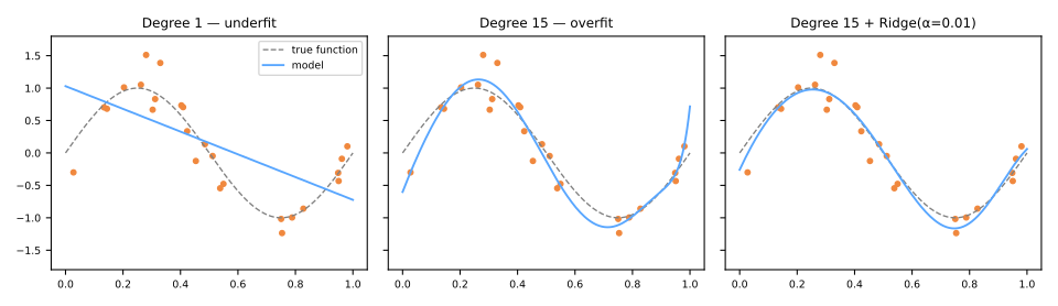
Degree 1 underfits — too rigid to follow the sine. Degree 15 overfits — 16 parameters chase 25 noisy points, producing wild oscillations. The right panel keeps all 16 parameters but adds a Ridge penalty: the curve relaxes back to the signal. That is regularization at work.

Underfitting and overfitting, measured

The figure convinces the eye. It is worth measuring, because the numbers show something the picture hides.

The data are 100 points of \(y = 0.5x^2 + x + 2\) with noise of standard deviation 3, for \(x\) between \(-3\) and \(3\). Three models: degree 1, degree 2 — the right degree — and degree 30. For each, the error on its own training set beside the error under five-fold cross-validation: the data are cut into five parts, the model is trained on four and scored on the fifth, and this is repeated so that each part is scored once. The five scores give a mean and a spread; the technique itself is the subject of the cross-validation lesson.

Degree 30 has the lowest training error of the three. Anyone picking a model by that column would pick the worst one.

The most instructive column, though, is the last. Look at the five folds of degree 30 one by one:

On three of the five it does as well as degree 2. On one, it explodes. Overfitting is not being wrong all the time — it is being wrong unpredictably, which is why the spread across folds gives the problem away before the mean does.

That yields a pocket diagnostic:

There is also a floor. The noise has standard deviation 3, and that part of \(y\) does not depend on \(x\), so no model can remove it. Degree 2 lands near that floor, which is all anyone can ask of a model.

Whether a degree is "too complex" also depends on how many points there are: section 11, in the advanced part, measures it.

6. Regularization

Stage 4. Instead of restricting the number of parameters, penalize their magnitude — add a complexity term to the loss:

Ridge (L2) — Tikhonov, 1943; Hoerl & Kennard, 1970

• shrinks all coefficients smoothly toward zero (never exactly zero);
• spreads weight across correlated features — the standard cure for multicollinearity;
• closed form still exists: \(\hat{w} = (X^\top X + \alpha I)^{-1} X^\top y\) — the \(\alpha I\) makes the matrix invertible even with collinear features.

Lasso (L1) — Tibshirani, 1996

• the absolute-value penalty has corners at zero: solutions land exactly at zero for weak features;
• performs automatic feature selection — the surviving nonzero coefficients name the features that matter;
• among a group of highly correlated features, it tends to keep one arbitrarily and zero the rest.

Elastic Net blends both penalties (l1_ratio) — a robust default when features are many and correlated.

from sklearn.linear_model import Ridge, Lasso, ElasticNet

Ridge(alpha=1.0)
Lasso(alpha=0.1)
ElasticNet(alpha=0.1, l1_ratio=0.5)

The one-dimensional case, in closed form

With a single feature, scaled so that \(\sum_i x_i^2 = 1\), the two penalties have explicit solutions, and you can derive them in two lines. The OLS coefficient is \(\hat{w} = \sum_i x_i y_i\), and the squared error is \(\sum_i (y_i - w x_i)^2 = \sum_i y_i^2 - 2w\hat{w} + w^2\). Add each penalty and set the derivative to zero:

The first gives a division; the second a subtraction, which only has a positive solution while \(\hat{w} > \alpha/2\) (otherwise the minimum sits at \(w = 0\)):

With \(\alpha = 1\):

Ridge divides; division never reaches zero. Lasso subtracts a fixed amount and clips at zero — so every coefficient below the threshold \(\alpha/2\) does not shrink, it disappears. That clipping is the automatic feature selection of the bullets above, written as a formula; section 12 shows its geometry.

The simulator fills this table one row at a time: step 0 derives the two formulas, each next step divides and subtracts for one row of the table, beside a plot of the penalized coefficient against the OLS one.

7. The knob α

\(\alpha\) trades data fidelity against coefficient size:

• \(\alpha \to 0\): plain OLS (no brake);
• \(\alpha \to \infty\): all coefficients crushed to ~0, model predicts the mean (full brake);
• the right \(\alpha\) is not known in advance — it is chosen by cross-validation (RidgeCV, LassoCV, or a grid search).

8. Summary: the engine and the brake in five lines

1. Gradient descent walks downhill: \(w \leftarrow w - \eta\,\nabla J\), with the gradient measured where you stand.
2. For the squared error, the gradient is a residual-weighted sum: \(-\frac{2}{n}\sum_i e_i\) for the intercept, \(-\frac{2}{n}\sum_i e_i x_i\) for the slope.
3. The learning rate decides the regime: too small creeps, too large diverges. Mini-batches make each step cheap.
4. Flexible models overfit: low training error, high and unpredictable validation error. The spread across folds gives it away.
5. Regularization penalizes the size of the coefficients: ridge divides them, lasso subtracts and clips them to zero; scale first, and choose \(\alpha\) by cross-validation.

Fundamental lab — downhill, one step at a time

The problem. Everything so far was a formula and a table computed by hand. This lab writes the update rule in a few lines of numpy, breaks it on purpose by pushing the learning rate, and trains a line on the three points of one step, by hand, checking every number of the table and the final answer against the closed form. No library does the descent for us: the point is to see the loop.

Step 1 — walk down a one-variable slope

Predict. The simplest possible loss, \(J(w) = (w-3)^2\), starting at \(w = 0\) with a fixed \(\eta = 0.1\). Will the steps all have the same size? Will \(w\) ever pass 3?

import numpy as np
import matplotlib.pyplot as plt


def J(w):
    return (w - 3) ** 2          # the loss: minimum at w = 3


def dJ(w):
    return 2 * (w - 3)           # its slope


w, eta = 0.0, 0.1                # initial guess and learning rate
print(f"{'step':>4} {'w':>8} {'J(w)':>9} {'dJ/dw':>8}")
for step in range(11):
    print(f"{step:>4} {w:>8.4f} {J(w):>9.4f} {dJ(w):>8.4f}")
    w = w - eta * dJ(w)

step        w      J(w)    dJ/dw
   0   0.0000    9.0000  -6.0000
   1   0.6000    5.7600  -4.8000
   2   1.0800    3.6864  -3.8400
   3   1.4640    2.3593  -3.0720
   4   1.7712    1.5099  -2.4576
   5   2.0170    0.9664  -1.9661
   6   2.2136    0.6185  -1.5729
   7   2.3709    0.3958  -1.2583
   8   2.4967    0.2533  -1.0066
   9   2.5973    0.1621  -0.8053
  10   2.6779    0.1038  -0.6442

The learning rate stayed at 0.1, yet the steps shrink on their own: 0.6, then 0.48, then 0.384, each one 0.8 times the previous. Near the bottom the slope is flatter, the derivative smaller, and the step, which is proportional to it, smaller too. After 10 steps \(w = 2.68\), still approaching from the left: nobody told the algorithm it was getting close.

Step 2 — the learning rate, pushed until it breaks

Predict. The same descent with \(\eta\) = 0.1, 0.5, 0.9 and 1.05. For each one: converges slowly, converges fast, bounces from side to side, or explodes?

def descend(w_start, eta, steps):
    ws = [w_start]
    for _ in range(steps):
        ws.append(ws[-1] - eta * dJ(ws[-1]))
    return np.array(ws)


for eta in [0.1, 0.5, 0.9, 1.05]:
    path = descend(0.0, eta, steps=12)
    print(f"eta = {eta:<4}  w after 1, 2, 3 steps: {np.round(path[1:4], 3)}  "
          f"after 12: {path[-1]:8.3f}  distance to 3: {abs(path[-1] - 3):.3f}")

fig, axes = plt.subplots(2, 2, figsize=(10, 6.5))
ws = np.linspace(-8, 14, 300)
for ax, eta in zip(axes.flat, [0.1, 0.5, 0.9, 1.05]):
    path = descend(0.0, eta, steps=12)
    ax.plot(ws, J(ws), lw=2)
    ax.plot(path, J(path), 'o-', ms=5, lw=1)
    ax.set_ylim(-5, 130); ax.set_title(f"eta = {eta}: w after 12 steps = {path[-1]:.3f}")
plt.tight_layout(); plt.show()

eta = 0.1   w after 1, 2, 3 steps: [0.6   1.08  1.464]  after 12:    2.794  distance to 3: 0.206
eta = 0.5   w after 1, 2, 3 steps: [3. 3. 3.]  after 12:    3.000  distance to 3: 0.000
eta = 0.9   w after 1, 2, 3 steps: [5.4   1.08  4.536]  after 12:    2.794  distance to 3: 0.206
eta = 1.05  w after 1, 2, 3 steps: [ 6.3   -0.63   6.993]  after 12:   -6.415  distance to 3: 9.415

Four behaviors with the same loss and the same algorithm. \(\eta = 0.1\) creeps in from the left. \(\eta = 0.5\) lands on 3 in one step and stays. \(\eta = 0.9\) jumps past the minimum to 5.4, comes back to 1.08, passes again, and still closes in. \(\eta = 1.05\) passes by more than it traveled: 6.3, −0.63, 6.993, farther each time, 9.4 away after 12 steps.

The algebra explains all four. Subtract 3 from both sides of the update:

The distance to the minimum is multiplied by \((1 - 2\eta)\) at every step: 0.8 for \(\eta = 0.1\), 0 for 0.5, −0.8 for 0.9 (it changes side but shrinks), −1.1 for 1.05 (it changes side and grows). That is also why \(\eta = 0.1\) and \(\eta = 0.9\) end at the same distance, 0.206: their factors have the same size, \(0.8^{12} \cdot 3 = 0.206\), one from each side.

Simulation: the boundary case. The factor \((1-2\eta)\) says the descent converges while \(0 < \eta < 1\). Before running anything, use it to predict what happens at exactly \(\eta = 1\), and just below and just above it. Then run descend with \(\eta\) = 0.95, 1.0 and 1.05 and print the first values of \(w\) and the distance to 3 after 12 steps.

for eta in [0.95, 1.0, 1.05]:
    path = descend(0.0, eta, steps=12)
    print(f"eta = {eta:<4}  w: {np.round(path[:6], 3)} ...  distance to 3 after 12 steps: {abs(path[-1] - 3):.3f}")

eta = 0.95  w: [0.    5.7   0.57  5.187 1.032 4.771] ...  distance to 3 after 12 steps: 0.847
eta = 1.0   w: [0. 6. 0. 6. 0. 6.] ...  distance to 3 after 12 steps: 3.000
eta = 1.05  w: [ 0.     6.3   -0.63   6.993 -1.392  7.832] ...  distance to 3 after 12 steps: 9.415

Step 3 — a line through three points

Predict. The three points of one step, by hand, now in code. Will the first rows printed match the hand table exactly? After 2000 iterations, will the loss reach zero?

x = np.array([1., 2., 3.])
y = np.array([2., 4., 7.])
X = np.column_stack([np.ones_like(x), x])           # column of ones + x
w_exact = np.linalg.solve(X.T @ X, X.T @ y)         # normal equations: the answer key
print(f"closed form: w0 = {w_exact[0]:.4f}   w1 = {w_exact[1]:.4f}")

closed form: w0 = -0.6667   w1 = 2.5000

The two derivatives of section 2 become two lines of code:

def loss(w0, w1, x, y):
    e = y - (w0 + w1 * x)
    return np.mean(e ** 2)


def gradient(w0, w1, x, y):
    n = len(x)
    e = y - (w0 + w1 * x)                           # residuals
    return -2 / n * np.sum(e), -2 / n * np.sum(e * x)


w0, w1, eta = 0.0, 0.0, 0.1
print(f"{'iter':>4} {'w0':>8} {'w1':>8} {'J':>8} {'dJ/dw0':>9} {'dJ/dw1':>9}")
for it in range(4):
    g0, g1 = gradient(w0, w1, x, y)
    print(f"{it:>4} {w0:>8.3f} {w1:>8.3f} {loss(w0, w1, x, y):>8.3f} {g0:>9.3f} {g1:>9.3f}")
    w0, w1 = w0 - eta * g0, w1 - eta * g1

iter       w0       w1        J    dJ/dw0    dJ/dw1
   0    0.000    0.000   23.000    -8.667   -20.667
   1    0.867    2.067    0.625     1.333     2.089
   2    0.733    1.858    0.344     0.231    -0.394
   3    0.710    1.897    0.327     0.343    -0.119

Row by row, the hand table of section 2. Now wrap the loop in a function that keeps the history, and let it run:

def train(x, y, eta, iterations, w0=0.0, w1=0.0):
    history = [(w0, w1, loss(w0, w1, x, y))]
    for _ in range(iterations):
        g0, g1 = gradient(w0, w1, x, y)
        w0, w1 = w0 - eta * g0, w1 - eta * g1
        history.append((w0, w1, loss(w0, w1, x, y)))
    return np.array(history)                        # columns: w0, w1, J


hist = train(x, y, eta=0.1, iterations=2000)
print(f"gradient descent: w0 = {hist[-1, 0]:.4f}   w1 = {hist[-1, 1]:.4f}   J = {hist[-1, 2]:.4f}")
print("J after 0, 1, 2, 3, 10, 100 iterations:", np.round(hist[[0, 1, 2, 3, 10, 100], 2], 3))

gradient descent: w0 = -0.6667   w1 = 2.5000   J = 0.0556
J after 0, 1, 2, 3, 10, 100 iterations: [23.     0.625  0.344  0.327  0.249  0.058]

Gradient descent reaches the closed form to four decimals. The first step removes almost all of the loss (23 → 0.625); the next 99 take it only from 0.625 to 0.058. And the loss does not reach zero: it stops at \(J = 0.0556\). Three points that are not aligned do not fit on a line, so an error is left that no \(w\) removes; reaching that floor is reaching the closed form.

Simulation: another starting point. Start the training from a terrible guess, \(w_0 = 10\) and \(w_1 = -10\), and from another one of your choice. Does the final answer change? Before running: how many minima do you think this loss has?

for start in [(0.0, 0.0), (10.0, -10.0), (-50.0, 30.0)]:
    h = train(x, y, eta=0.1, iterations=2000, w0=start[0], w1=start[1])
    print(f"start {str(start):>13}: J at start {h[0, 2]:9.1f} -> w0 = {h[-1, 0]:.4f}  w1 = {h[-1, 1]:.4f}  J = {h[-1, 2]:.4f}")

start    (0.0, 0.0): J at start      23.0 -> w0 = -0.6667  w1 = 2.5000  J = 0.0556
start (10.0, -10.0): J at start     309.7 -> w0 = -0.6667  w1 = 2.5000  J = 0.0556
start (-50.0, 30.0): J at start     536.3 -> w0 = -0.6667  w1 = 2.5000  J = 0.0556

To close the fundamental part. In one sentence each: (1) why do the steps shrink near the minimum even with a fixed \(\eta\)? (2) Why does a learning rate slightly above the threshold diverge instead of converging slowly? (3) Why does lasso set a weak coefficient exactly to zero while ridge only makes it smaller?

Your turn (fundamental)

At home:

1. Iteration 4 by hand. From the last row of the step-3 table (\(w_0 = 0.710\), \(w_1 = 1.897\)), compute the residuals, the two derivatives and the update with a calculator. Then run the loop with range(5) and check.
2. A ten times smaller learning rate. Train the three points with \(\eta = 0.01\) for 2000 iterations. How far from the closed form does it stop? How many iterations would it need?
3. Ridge and lasso with a stronger brake. Redo the one-dimensional table of section 6 with \(\alpha = 2\). Which coefficients survive the lasso? What fraction of each one does ridge keep?

Advanced approach

The fundamental part derived the gradient for a line, tuned the step and put a brake on a flexible model. This part looks inside both tools: what the gradient looks like with any number of features, why the shape of the loss surface — and so the scale of the features — decides whether the descent works, why "too complex" depends on the amount of data, and why lasso zeroes coefficients that ridge only shrinks. The code blocks continue those of the fundamental lab.

This part follows one path in four stages, drawn below: 1. any number of parameters; 2. read the landscape; 3. complexity is relative; 4. inside the penalties. Each stage links to its section, and in the slides a strip at the bottom shows which stage you are in.

Advanced approach slides

Click the slides and use the ← → arrows to navigate; F opens full screen and Esc shows every slide. Open the slides in a new tab

9. The gradient for any number of parameters

Stage 1. Section 2 derived two derivatives, one for the intercept and one for the slope. A model with \(d\) features has \(d+1\) of them, and writing them one by one does not scale. It does not have to: they all have the same shape.

And so on: parameter \(j\)

With \(d\) features the model is \(\hat{y}_i = w_0 + w_1x_{i1} + \dots + w_dx_{id}\). Adopt the convention \(x_{i0} = 1\) — the column of ones already sitting in the design matrix — and the intercept stops being a special case: it becomes just the weight on a constant column. The derivative of the residual then always has the same shape,

and a single formula covers every parameter:

Notice the first row is not an exception to the last: it is the last, with \(x_{i0}=1\). It is the same column-of-ones trick that turned \(\hat{y} = w_0 + w_1x\) into \(\hat{y} = Xw\).

Stacking them: the matrix form

Now collect those \(d+1\) derivatives into a vector. Entry \(j\) is \(\sum_i e_i x_{ij}\), which is the \(j\)-th column of \(X\) dotted with the residual vector. Doing that for every column at once is multiplying by \(X^\top\):

There is no magic in this formula: it is the table above, written compactly. That is why one line of numpy computes the gradient of a model with a million parameters — the structure is exactly the one for \(w_0\) and \(w_1\), repeated. Step 5 of the lab writes that line.

Two readings come out of this, and both travel far.

First: set the gradient to zero and you recover the normal equations, \(X^\top(y - Xw) = 0\) — which is the closed-form solution from last lesson. The closed form and the gradient are the same statement by two routes: one solves \(\nabla J = 0\) in a single move, the other walks there.

Second: look at what the gradient is made of — a residual-weighted sum. A point the model already predicts well enters with \(e_i \approx 0\) and barely votes; a point it badly misses dominates the step. So the rule \(w \leftarrow w - \eta\,\nabla J\) reads, in plain words: move each weight in the direction the errors point, by an amount proportional to how large those errors are. That sentence stays true, word for word, when the model is a 100-layer network and \(\nabla J\) comes from backpropagation.

10. The landscape you are walking down

Stage 2. So far the descent has been numbers in a table. It is worth seeing what they are geometrically, because the picture explains both the slowness of the hand table and its cure at once.

Think of \(J(w_0, w_1)\) as a landscape: every point of the plane is a pair of weights, that is, a candidate line, and the height there is the error that line makes. Minimizing means hunting for the bottom of the valley. The gradient is the direction of steepest ascent at that point, so \(-\nabla J\) is the direction of steepest descent.

The simulator that closed the previous lesson draws it; now you can read it with the table in hand. The left panel shows the contours of that landscape, with the closed-form optimum marked. On the right, the same weights drawn as a line through the data. Click on the left to drop a starting guess, then keep pressing Step:

Now switch on center x and start again from a similar point. Same data, same algorithm, completely different behavior.

Uncentered, the contours form a long, narrow valley. The reason is the asymmetry you saw in the hand table: \(w_0\) and \(w_1\) become coupled, because tilting a line whose \(x\) values all sit far from zero also raises or lowers its height. The gradient points across the valley instead of along it, so the path zigzags and drags. Centered, the valley becomes a round bowl and the same steps go nearly straight to the answer. Step 4 of the lab counts the iterations each version needs, and finds where each one breaks.

11. "Too complex" is relative to how much data you have

Stage 3. Section 5 measured overfitting on 100 points. Complexity is not a property of the model alone: it is the relationship between the number of parameters and the number of points.

A degree-10 polynomial has 11 free parameters — ten powers plus the intercept. As long as the training points do not outnumber those, the curve can pass exactly through every one of them:

Zero training error is not a sign of success: it is a sign that nothing was left over. With ten points and eleven parameters the model never had to learn anything about the shape of the curve — memorizing was enough. From the eleventh point on it has to start choosing, and the training error lifts off the floor.

Notice what this implies: the same degree-10 model is too complex for 10 points and perfectly reasonable for 100. There is no "right" degree in the abstract, only a right degree for a quantity of data. The tool that makes this dependence visible is the learning curve — training and validation error against training-set size — covered in model selection.

12. Why L1 zeroes and L2 does not

Stage 4. The bullet lists of section 6 assert the difference, and the one-dimensional formula shows it for a single coefficient. With two or more coefficients the reason is geometric, and it is worth seeing rather than believing.

Write the penalty as a budget instead: minimize the squared error subject to \(\sum |w_j| \le t\) (lasso) or \(\sum w_j^2 \le t^2\) (ridge). The two formulations are equivalent — every \(\alpha\) has a matching \(t\). Now the picture is two objects: the elliptical contours of the error, centered on the OLS solution, and the feasible region.

The constrained solution is where the ellipse, growing outward from the OLS optimum, first touches the region:

The circle has no corners, so the touch point can be anywhere on it — and lands on an axis only by coincidence. The diamond has four corners, and they sit exactly on the axes. A smooth curve expanding toward a pointed region tends to meet a point first, and meeting a corner is a coefficient being exactly zero.

Drag the OLS optimum around and watch how often the diamond is touched at a corner while the circle almost never is. Lasso does not select features by thresholding — it selects them because of the shape of its constraint. The subtraction-and-clip of the one-dimensional case is that corner, written as a formula.

13. Watching the path

Run the penalty across a range of \(\alpha\) and plot every coefficient. Eight features here: three carry real signal, three are pure noise, and two are near-copies of each other.

Lasso removes the noise features first — exactly the selection you hoped for — and the count keeps dropping. Ridge never drops below eight at any \(\alpha\): the noise coefficients get small and stay.

Then switch to the correlated pair \(c_1, c_2\), whose true coefficients are both 2. At \(\alpha = 2\) lasso reports (1.89, 0.98) — it is starting to pick one and discard the other, and which one is close to arbitrary. Ridge reports (1.02, 0.97): it splits the weight evenly. That is the whole reason ridge is the standard answer to multicollinearity and lasso is not.

14. Practical profile

Advanced lab — scale, many features and mini-batches

The fundamental lab trained a line on three points and saw the learning rate break the descent. This part looks at the landscape of those same three points with and without centering, writes the gradient in one line, takes it to 20,640 California districts where the scale of the features decides everything, puts the ridge penalty inside the loop, and replaces the full dataset with small batches. Continue in the same notebook, in the same session: the steps below use x, y, X, w_exact, gradient and train from steps 1 to 3.

Step 4 — the landscape, with and without centering

Predict. The same three points, once with \(x = 1, 2, 3\) and once centered, \(x - \bar{x} = -1, 0, 1\). Same \(\eta\), same start. Which version needs fewer iterations? With \(\eta = 0.5\), which one converges at all?

def contour_map(ax, x, y, hist, title):
    X = np.column_stack([np.ones_like(x), x])
    w_opt = np.linalg.solve(X.T @ X, X.T @ y)
    W0, W1 = np.meshgrid(np.linspace(w_opt[0] - 4, w_opt[0] + 4, 200),
                         np.linspace(w_opt[1] - 3.5, w_opt[1] + 3.5, 200))
    E = y[:, None, None] - (W0 + W1 * x[:, None, None])
    ax.contour(W0, W1, np.mean(E ** 2, axis=0), levels=np.geomspace(0.06, 60, 14), linewidths=.8)
    ax.plot(hist[:, 0], hist[:, 1], 'o-', ms=3, lw=1)
    ax.plot(*w_opt, '*', ms=15)
    ax.set_xlabel('w0 (intercept)'); ax.set_ylabel('w1 (slope)'); ax.set_title(title)


x_c = x - x.mean()                                  # centered: -1, 0, 1
fig, (ax1, ax2) = plt.subplots(1, 2, figsize=(11, 4.5))
contour_map(ax1, x, y, train(x, y, 0.1, 30), 'original x: a narrow valley')
contour_map(ax2, x_c, y, train(x_c, y, 0.1, 30), 'centered x: almost a round bowl')
plt.tight_layout(); plt.show()


def iterations_to_converge(x, y, eta, tol=1e-3, limit=10_000):
    X = np.column_stack([np.ones_like(x), x])
    w_opt = np.linalg.solve(X.T @ X, X.T @ y)
    w0 = w1 = 0.0
    for it in range(limit):
        if max(abs(w0 - w_opt[0]), abs(w1 - w_opt[1])) < tol:
            return f"{it} iterations"
        if abs(w0) + abs(w1) > 1e6:
            return "DIVERGED"
        g0, g1 = gradient(w0, w1, x, y)
        w0, w1 = w0 - eta * g0, w1 - eta * g1
    return f"not there in {limit}"


print(f"{'eta':>5}   {'original x':>16}   {'centered x':>16}")
for eta in [0.05, 0.1, 0.15, 0.2, 0.5]:
    print(f"{eta:>5}   {iterations_to_converge(x, y, eta):>16}   {iterations_to_converge(x_c, y, eta):>16}")

  eta         original x         centered x
 0.05     604 iterations     114 iterations
  0.1     300 iterations      55 iterations
 0.15     199 iterations      36 iterations
  0.2           DIVERGED      26 iterations
  0.5           DIVERGED       8 iterations

On the left map, the contours form a long, tilted valley: the first step crosses it at once and the path then drags along its floor, and after 30 steps it has not reached the star. On the right, almost circles, and the path goes nearly straight. The table puts numbers on it: at every \(\eta\) the centered version needs about five times fewer iterations, and it tolerates learning rates that make the original diverge: at \(\eta = 0.5\) it converges in 8 iterations, while the original already breaks at 0.2. The closed form returns the same line in both cases; gradient descent depends entirely on the scale of the data.

Simulation: where the limit sits. Find, to two decimals, the largest \(\eta\) that still converges for the original \(x\) and for the centered one (scan \(\eta\) from 0.01 upward with iterations_to_converge). How many times larger is the limit after centering? Then compute the eigenvalues of \(\tfrac{2}{n}X^\top X\), the curvatures of the loss along its two main directions, and compare 2 divided by the largest one with the limits you found. Step 2 had a curvature too: which?

for name, xs in [('original', x), ('centered', x_c)]:
    etas = np.round(np.arange(0.01, 1.30, 0.01), 2)
    ok = [eta for eta in etas if 'iterations' in iterations_to_converge(xs, y, eta)]
    H = 2 / len(xs) * np.column_stack([np.ones_like(xs), xs]).T @ np.column_stack([np.ones_like(xs), xs])
    lam = np.linalg.eigvalsh(H)
    print(f"{name:>8} x: largest eta that converges = {max(ok):.2f} · "
          f"curvatures {lam.round(3)} · 2 / largest = {2 / lam.max():.3f} · ratio {lam.max() / lam.min():.1f}")

original x: largest eta that converges = 0.18 · curvatures [ 0.24  11.093] · 2 / largest = 0.180 · ratio 46.1
centered x: largest eta that converges = 0.99 · curvatures [1.333 2.   ] · 2 / largest = 1.000 · ratio 1.5

Step 5 — many features: the gradient in one line, on 20,640 districts

Predict. The matrix form of section 9 fits in one line of code. On California houses, with features whose values go from units (income) to tens of thousands (total rooms), will the \(\eta = 0.01\) that worked on three points still work?

The matrix version first, checked on the three points:

def gd(X, y, eta, iterations):
    n, d = X.shape
    w = np.zeros(d)
    losses = []
    for _ in range(iterations):
        e = y - X @ w
        losses.append(np.mean(e ** 2))
        w = w - eta * (-2 / n) * X.T @ e            # w <- w - eta * gradient
    return w, np.array(losses)


w, _ = gd(X, y, eta=0.1, iterations=2000)
print("matrix version:", w.round(4), "· closed form:", w_exact.round(4))

matrix version: [-0.6667  2.5   ] · closed form: [-0.6667  2.5   ]

The same function works for any number of columns. The California housing data: 20,640 census districts of 1990, the median house value (in units of $100,000) predicted from four features. Look at the scales before anything else:

import pandas as pd

url = "https://raw.githubusercontent.com/hsandmann/biblio/refs/heads/main/ml/aula03/housing.csv"
df = pd.read_csv(url)
features = ['median_income', 'housing_median_age', 'total_rooms', 'population']
A = df[features].to_numpy(dtype=float)
target = df['median_house_value'].to_numpy(dtype=float) / 1e5     # in $100,000
print(df[features].describe().loc[['mean', 'std', 'min', 'max']].round(1))

X_raw = np.column_stack([np.ones(len(A)), A])
w_ref = np.linalg.lstsq(X_raw, target, rcond=None)[0]             # least squares: the answer key
rmse_ref = np.sqrt(np.mean((target - X_raw @ w_ref) ** 2))
print(f"RMSE of the best possible linear fit (answer key): {rmse_ref:.4f}")

      median_income  housing_median_age  total_rooms  population
mean            3.9                28.6       2635.8      1425.5
std             1.9                12.6       2181.6      1132.5
min             0.5                 1.0          2.0         3.0
max            15.0                52.0      39320.0     35682.0
RMSE of the best possible linear fit (answer key): 0.8021

Income has a standard deviation of 1.9; total rooms, of 2,181.6, and a maximum of 39,320. Now the descent on the raw features, and then with a learning rate small enough not to explode:

with np.errstate(over='ignore', invalid='ignore'):
    w, losses = gd(X_raw, target, eta=0.01, iterations=10)
print("eta = 0.01, raw features, J per iteration:", [f"{v:.3g}" for v in losses])

w, losses = gd(X_raw, target, eta=1e-8, iterations=1000)
print(f"eta = 1e-8, raw features: RMSE after 1000 iterations {np.sqrt(losses[-1]):.4f} · "
      f"income weight {w[1]:.5f} (answer key {w_ref[1]:.5f})")

eta = 0.01, raw features, J per iteration: ['5.61', '2.48e+11', '2.15e+22', '1.87e+33', '1.62e+44', '1.41e+55', '1.22e+66', '1.06e+77', '9.19e+87', '7.97e+98']
eta = 1e-8, raw features: RMSE after 1000 iterations 1.6475 · income weight 0.00008 (answer key 0.41272)

With \(\eta = 0.01\) the loss goes from 5.61 to \(10^{98}\) in ten iterations: the gradient along total_rooms is gigantic, and any reasonable step for income is an absurd leap for rooms. Lowering \(\eta\) to \(10^{-8}\) stops the explosion but also stops the learning: after 1000 iterations the RMSE is 1.65, twice the answer key, and the income weight, the feature that matters most, has barely left zero (0.00008 against 0.41272). It is the narrow valley of step 4, now in five dimensions. The cure is the one of step 4 as well: give every column mean 0 and standard deviation 1.

Z = (A - A.mean(axis=0)) / A.std(axis=0)            # mean 0, standard deviation 1
X_std = np.column_stack([np.ones(len(Z)), Z])
w, losses = gd(X_std, target, eta=0.1, iterations=200)
w_ref_std = np.linalg.lstsq(X_std, target, rcond=None)[0]
print(f"eta = 0.1, standardized: RMSE after 200 iterations {np.sqrt(losses[-1]):.4f} (answer key {rmse_ref:.4f})")
print("RMSE after 5, 10, 20, 50 iterations:", np.sqrt(losses[[5, 10, 20, 50]]).round(4))
print("weights, gradient descent:", w.round(4))
print("weights, answer key:      ", w_ref_std.round(4))

eta = 0.1, standardized: RMSE after 200 iterations 0.8021 (answer key 0.8021)
RMSE after 5, 10, 20, 50 iterations: [1.0897 0.8396 0.8031 0.8022]
weights, gradient descent: [ 2.0686  0.7842  0.2493  0.2025 -0.1318]
weights, answer key:       [ 2.0686  0.7841  0.2494  0.2032 -0.1325]

Same data, same algorithm, same code; only the scale of the columns changed, and the method went from "explodes or does not move" to the answer key's RMSE, 0.8031 after only 20 iterations. With standardized columns the weights can be compared: income dominates (0.784) and population enters with a negative sign. Here the whole dataset was standardized because the subject is optimization; in a real model the mean and standard deviation come from the training set only, inside a pipeline.

Simulation: the brake inside the engine. Add the ridge penalty to the loss, \(J = \frac{1}{n}\sum_i e_i^2 + \alpha\sum_{j \ge 1} w_j^2\): its gradient gains a term \(2\alpha w_j\) for every weight except the intercept. Write gd_ridge, run it on the standardized California data with \(\alpha\) = 0, 0.1, 1 and 10, and print the four weights and the training RMSE. What happens to the weights, and does any of them reach exactly zero? Finally, compare with scikit-learn's Ridge: which alpha must you pass it to get the same weights?

from sklearn.linear_model import Ridge

def gd_ridge(X, y, eta, iterations, alpha):
    n, d = X.shape
    w = np.zeros(d)
    for _ in range(iterations):
        e = y - X @ w
        penalty = 2 * alpha * w
        penalty[0] = 0                               # the intercept is not penalized
        w = w - eta * ((-2 / n) * X.T @ e + penalty)
    return w

n = len(target)
for alpha in [0, 0.1, 1, 10]:
    w_r = gd_ridge(X_std, target, eta=0.05, iterations=2000, alpha=alpha)
    sk = Ridge(alpha=n * alpha).fit(Z, target) if alpha > 0 else None
    print(f"alpha = {alpha:<4} weights {w_r[1:].round(4)}  RMSE {np.sqrt(np.mean((target - X_std @ w_r) ** 2)):.4f}"
          + (f"  sklearn Ridge(alpha={n * alpha:g}): {sk.coef_.round(4)}" if sk is not None else ""))

alpha = 0    weights [ 0.7841  0.2494  0.2032 -0.1325]  RMSE 0.8021
alpha = 0.1  weights [ 0.7181  0.2142  0.1513 -0.0892]  RMSE 0.8063  sklearn Ridge(alpha=2064): [ 0.7181  0.2142  0.1513 -0.0892]
alpha = 1    weights [ 0.3958  0.0922  0.068  -0.0307]  RMSE 0.9077  sklearn Ridge(alpha=20640): [ 0.3958  0.0922  0.068  -0.0307]
alpha = 10   weights [ 0.0721  0.0122  0.0134 -0.0033]  RMSE 1.1024  sklearn Ridge(alpha=206400): [ 0.0721  0.0122  0.0134 -0.0033]

Step 6 — mini-batch: cheap steps

Predict. Every iteration of step 5 goes through all 20,640 rows to take one step. With the same cost, one pass over the data, you can instead take 645 steps of 32 rows each. Who ends closer to the answer key after that one pass? And what will the mini-batch curve look like near the floor?

def minibatch_gd(X, y, eta, epochs, batch_size, seed=0):
    rng = np.random.default_rng(seed)
    n, d = X.shape
    w = np.zeros(d)
    losses = []
    for _ in range(epochs):
        order = rng.permutation(n)                  # reshuffle every epoch
        for start in range(0, n, batch_size):
            batch = order[start:start + batch_size]
            e = y[batch] - X[batch] @ w
            w = w - eta * (-2 / len(batch)) * X[batch].T @ e
            losses.append(np.mean((y - X @ w) ** 2))   # J on the whole set, only to plot
    return w, np.array(losses)


w_mb, losses_mb = minibatch_gd(X_std, target, eta=0.01, epochs=1, batch_size=32)
w_batch, _ = gd(X_std, target, eta=0.1, iterations=1)
rmse_batch = np.sqrt(np.mean((target - X_std @ w_batch) ** 2))
print("after ONE pass over the data:")
print(f"  {'batch GD, 1 step':<26} RMSE = {rmse_batch:.4f}")
print(f"  {f'mini-batch, {len(losses_mb)} steps':<26} RMSE = {np.sqrt(losses_mb[-1]):.4f}")
print(f"  {'answer key':<26} RMSE = {rmse_ref:.4f}")
print("RMSE over the last 100 steps: min", np.sqrt(losses_mb[-100:]).min().round(4), "max", np.sqrt(losses_mb[-100:]).max().round(4))

after ONE pass over the data:
  batch GD, 1 step           RMSE = 1.9568
  mini-batch, 645 steps      RMSE = 0.8024
  answer key                 RMSE = 0.8021
RMSE over the last 100 steps: min 0.8023 max 0.8045

For the price of one batch iteration — one pass over the data — the mini-batch is already at 0.8024, against 0.8021 for the answer key, while the single batch step is still at 1.9568. The price shows in the last line: over its final 100 steps the RMSE trembles between 0.8023 and 0.8045 instead of settling on the floor, because each step sees only 32 houses and each batch pulls a little to its own side. Cheap and noisy, but heading the right way. This loop, with other losses in place of the squared error, is what trains logistic regression, SVMs and neural networks.

To close the lesson. In one sentence each: (1) why does centering the three points allow a learning rate five times larger? (2) Why does \(\eta = 0.01\) explode on the raw California features but not on the standardized ones? (3) Why does the mini-batch curve tremble around the floor instead of settling on it?

Your turn (advanced)

At home, with more time:

1. All the features. In step 5, replace features with every numeric column except the target. One of them has missing values: drop those rows with df = df.dropna() before building A. Does the answer key's RMSE improve? Does the standardized gradient descent still reach it with \(\eta = 0.1\)?
2. Batch size. In step 6, run minibatch_gd with batch_size equal to 1, 32 and 1024, one epoch each, and plot the three curves. Which trembles most? Which gets closest to the answer key in one pass? With batch_size=1 you may need to lower \(\eta\): why?
3. Lasso by gradient descent. In gd_ridge, replace the penalty \(2\alpha w_j\) with \(\alpha\,\operatorname{sign}(w_j)\), the slope of \(\alpha|w_j|\), and run it with \(\alpha = 0.1\) and \(\alpha = 0.3\). Does any weight reach exactly zero, or do some of them jitter around it? Relate what you see to the subtract-and-clip formula of section 6, which is what lasso solvers apply instead.

References

• Tikhonov, A. N. "On the stability of inverse problems." C. R. (Doklady) Acad. Sci. URSS, n. Ser. 39 (1943), 176–179. zbMATH record
• Robbins, H.; Monro, S. "A Stochastic Approximation Method." Annals of Math. Statistics 22 (1951). DOI
• Hoerl, A. E.; Kennard, R. W. "Ridge Regression: Biased Estimation for Nonorthogonal Problems." Technometrics 12 (1970). DOI
• Tibshirani, R. "Regression Shrinkage and Selection via the Lasso." JRSS B 58 (1996). DOI

Quiz