Why the closed form is not enough
The closed form of ordinary least squares (OLS), \(\hat w = (X^\top X)^{-1}X^\top y\), solves linear regression in one move. But:
it does not scale
inverting \(X^\top X\) costs \(O(d^3)\) for \(d\) features: hopeless with huge feature counts
it does not exist
for most other models, starting with neural networks
it does not brake
it says nothing about controlling overfitting
The path of this part
- Walk downhillthe gradient, derived and computed by hand
- Tune the stepthe learning rate; batch, stochastic, mini-batch
- Lines → curvespolynomial features; underfitting and overfitting
- Regularizeridge (L2), lasso (L1) and the knob α
Gradient descent: walk downhill
Instead of solving \(\nabla J = 0\) on paper: measure the slope where you stand, step against it, repeat.
\[ w^{(t+1)} = w^{(t)} - \eta \, \nabla_w J\big(w^{(t)}\big) \]- \(J(w)\): the loss, the error the model makes with weights \(w\); \(t\): the iteration.
- \(\eta\): the learning rate, the size of the step.
- \(\nabla_w J\), the gradient, points where the loss grows fastest; the minus sign makes the method descend.
Where the gradient comes from
\[ J(w_0, w_1) = \frac{1}{n}\sum_{i=1}^{n}\big(\underbrace{y_i - w_0 - w_1 x_i}_{e_i}\big)^2 \]\(n\) points \((x_i, y_i)\); \(e_i\) is the residual of point \(i\). Chain rule: the derivative of \(e_i^2\) is \(2e_i\) times how the residual reacts to the weight.
\(\partial e_i / \partial w_0 = -1\)
raising the intercept by one lowers every residual by one
\(\partial e_i / \partial w_1 = -x_i\)
raising the slope lowers the residual by \(x_i\): points far from the origin feel it more
Gradient descent, by hand
Points \((1,2), (2,4), (3,7)\); start at \(w_0 = w_1 = 0\); \(\eta = 0.1\). Predict. Which way will the first step move each weight, and how much of the loss of 23 will it remove?
The learning rate
- \(\eta\) too small → tiny steps, slow convergence
- \(\eta\) too large → the steps overshoot; the loss oscillates or diverges
- recipe: try \(\eta \in \{10^{-3}, 10^{-2}, 10^{-1}\}\) and watch the training loss fall smoothly
On \(J(w) = (w-3)^2\), slope \(2(w-3)\), subtract 3 from both sides of the update:
\[ w_{t+1} - 3 = (1 - 2\eta)\,(w_t - 3) \]the distance to the minimum is multiplied by \(1 - 2\eta\) at every step.
so, on this loss
| \(\eta < 0.5\) | creeps in |
| \(\eta = 0.5\) | the minimum in one move |
| \(0.5 < \eta < 1\) | bounces, but closes in |
| \(\eta = 1\) | bounces between two points for ever |
| \(\eta > 1\) | explodes |
Simulator: the learning rate
Predict. Set \(\eta = 1.05\) and step through it. Does it converge, bounce for ever or explode?
Batch, stochastic and mini-batch
The gradient sums over all \(n\) points: with millions of rows, one step costs a full pass over the data.
| variant | gradient computed on | cost per step | behavior |
|---|---|---|---|
| batch gradient descent (GD) | the full dataset | \(O(nd)\) | exact, smooth descent |
| stochastic GD (SGD) | one random sample | \(O(d)\) | noisy but cheap; escapes shallow traps |
| mini-batch GD | a batch of ~32–512 | in between | the modern default |
from sklearn.linear_model import SGDRegressor
model = SGDRegressor(loss='squared_error', penalty='l2', alpha=1e-4,
                     learning_rate='invscaling', max_iter=1000)
From lines to curves: polynomial features
Linear regression is linear in the parameters, not in the inputs: \(x \mapsto (x, x^2, \dots, x^p)\), and the same OLS fits the weights.
from sklearn.pipeline import make_pipeline
from sklearn.preprocessing import PolynomialFeatures

model = make_pipeline(PolynomialFeatures(degree=3), LinearRegression())
Flexibility cuts both ways
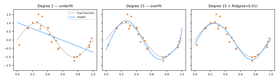
Degree 1 underfits: too rigid. Degree 15 overfits: 16 parameters chase 25 noisy points. Right: the same 16 parameters plus a Ridge penalty, and the curve relaxes back to the signal.
Underfitting and overfitting, measured
100 points of \(y = 0.5x^2 + x + 2\), noise with standard deviation 3; five-fold cross-validation. RMSE: root mean squared error, in units of \(y\).
| degree | train RMSE | validation RMSE (mean) | spread across folds |
|---|---|---|---|
| 1 | 3.22 | 3.26 | 0.19 |
| 2 | 2.64 | 2.75 | 0.33 |
| 30 | 2.46 | 10.43 | 13.46 |
Degree 30, fold by fold: \(3.14 \quad 3.02 \quad 5.51 \quad \mathbf{37.29} \quad 3.20\)
A pocket diagnostic
| too simple (underfitting) | too complex (overfitting) | |
|---|---|---|
| training error | high | low |
| validation error | high, consistently | high on average, occasionally low |
| spread across folds | small | large |
| what to do | more capacity, better features | regularize, more data, less capacity |
Regularization: penalize the magnitude
Ridge (L2) · Tikhonov 1943; Hoerl & Kennard 1970
\[ \lVert y - Xw \rVert^2 + \alpha \sum_j w_j^2 \]- shrinks smoothly, never to exactly zero
- spreads weight across correlated features
- closed form: \((X^\top X + \alpha I)^{-1} X^\top y\)
Lasso (L1) · Tibshirani 1996
\[ \lVert y - Xw \rVert^2 + \alpha \sum_j \lvert w_j \rvert \]- lands exactly at zero for weak features
- automatic feature selection
- among correlated features, keeps one arbitrarily
\(\lVert y - Xw\rVert^2\): the sum of squared errors; \(\alpha \ge 0\): the strength of the penalty. L2 penalizes the sum of squares of the weights, L1 the sum of their absolute values. Elastic Net blends both (l1_ratio).
Ridge and lasso on one coefficient, by hand
One feature, \(\sum x_i^2 = 1\), \(\alpha = 1\); \(\hat w\) is the OLS coefficient. Predict. Which penalty can turn \(\hat w = 0.2\) into exactly zero, and why?
The knob α
- \(\alpha \to 0\): plain OLS, no brake.
- \(\alpha \to \infty\): every coefficient crushed to ~0, the model predicts the mean.
- The right \(\alpha\) is not known in advance: choose it by cross-validation (
RidgeCV,LassoCV, a grid search).
Summary
- Gradient descent walks downhill: \(w \leftarrow w - \eta\nabla J\).
- For the squared error the gradient is a residual-weighted sum: \(-\frac{2}{n}\sum e_i\), \(-\frac{2}{n}\sum e_i x_i\).
- \(\eta\) too large diverges, too small creeps; mini-batches make each step cheap.
- Overfitting = low training error, high and unpredictable validation error.
- Ridge divides the coefficients, lasso subtracts and clips them to zero; scale first, choose \(\alpha\) by cross-validation.
| symptom | what to do |
|---|---|
| the loss grows at every step | divide \(\eta\) by 10 |
| training error far below validation, folds that disagree | regularize, more data, less capacity |
Downhill, one step at a time, steps 1 to 3
- Step 1: walk down \(J(w) = (w-3)^2\) with a fixed \(\eta\). Step 2: push \(\eta\) until it breaks. Step 3: train a line on the three points of the hand table and check every number against the closed form.
- Notebook on Colab (in Portuguese), sections 1 to 3: nothing to download. Save a copy to your Drive.
- At every step, answer the Predict before running.
- Simulations: the boundary case (step 2) and another starting point (step 3).
Pace: steps 1 and 2 and the first simulation in 12 min; step 3 and the second in 13 min.