Why the closed form is not enough
it does not scale
\((X^\top X)^{-1}\) costs \(O(d^3)\): hopeless with huge feature counts
it does not exist
for most other models, starting with neural networks
it does not brake
it says nothing about controlling overfitting
The path of this lesson
- Walk downhillthe gradient, derived and computed by hand
- Tune the descentloss landscape, scaling, learning rate, batches
- Lines → curvespolynomial features; underfitting and overfitting
- Regularizeridge (L2), lasso (L1) and the knob α
Gradient descent: walk downhill
Instead of solving \(\nabla J = 0\) on paper: measure the slope where you stand, step against it, repeat.
\[ w^{(t+1)} = w^{(t)} - \eta \, \nabla_w J\big(w^{(t)}\big) \]- \(\eta\): the learning rate, the size of the step.
- \(\nabla_w J\) points where the loss grows fastest; the minus sign makes the method descend.
Where the gradient comes from
\[ J(w_0, w_1) = \frac{1}{n}\sum_{i=1}^{n}\big(\underbrace{y_i - w_0 - w_1 x_i}_{e_i}\big)^2 \]Chain rule: the derivative of \(e_i^2\) is \(2e_i\) times how the residual reacts to the weight.
\(\partial e_i / \partial w_0 = -1\)
raising the intercept by one lowers every residual by one
\(\partial e_i / \partial w_1 = -x_i\)
raising the slope lowers the residual by \(x_i\): points far from the origin feel it more
One formula for every parameter
With the column of ones \(x_{i0} = 1\), the intercept is just one more weight:
\[ \frac{\partial J}{\partial w_j} = -\frac{2}{n}\sum_{i=1}^{n} e_i\,x_{ij} \qquad\Longrightarrow\qquad \nabla_w J = -\frac{2}{n}X^\top e = -\frac{2}{n}X^\top(y - Xw) \]first reading
set it to zero: \(X^\top(y - Xw) = 0\), the normal equations. Same statement, two routes: solve it at once, or walk there.
second reading
a residual-weighted sum: well-predicted points barely vote, badly missed points dominate the step.
One step, by hand
Points \((1,2), (2,4), (3,7)\); start at \(w_0 = w_1 = 0\); \(\eta = 0.1\).
The line predicts 0 everywhere, so \(e = y = (2, 4, 7)\): \(\sum e_i = 13\), \(\sum e_i x_i = 2 + 8 + 21 = 31\).
\[ \frac{\partial J}{\partial w_0} = -\tfrac{2}{3}(13) = -8.667, \qquad \frac{\partial J}{\partial w_1} = -\tfrac{2}{3}(31) = -20.667 \] \[ w_0 \leftarrow 0 - 0.1(-8.667) = 0.867, \qquad w_1 \leftarrow 0 - 0.1(-20.667) = 2.067 \]The next steps
| iteration | \(w_0\) | \(w_1\) | \(J\) | \(\partial J/\partial w_0\) | \(\partial J/\partial w_1\) |
|---|---|---|---|---|---|
| 0 | 0.000 | 0.000 | 23.000 | −8.667 | −20.667 |
| 1 | 0.867 | 2.067 | 0.625 | 1.333 | 2.089 |
| 2 | 0.733 | 1.858 | 0.344 | 0.231 | −0.394 |
| 3 | 0.710 | 1.897 | 0.327 | 0.343 | −0.119 |
first step enormous
23 → 0.63, then it crawls: a fast early fall says little about convergence
signs flip
a step overshoots the minimum, the next walks it back
uneven pace
\(\partial J/\partial w_1\) is 2.4× \(\partial J/\partial w_0\): residuals enter multiplied by \(x_i\)
After 2000 iterations: \(w_0 = -0.667\), \(w_1 = 2.5\), exactly the normal equations.
The landscape you are walking down
- Every point of the plane \((w_0, w_1)\) is a candidate line; the height is its error.
- Minimizing = finding the bottom of the valley; \(-\nabla J\) is the direction of steepest descent.
Simulator: the loss surface
Click on the left to drop a start and press Step. Then switch center x on and start again from a similar point.
Why scaling comes before fitting
uncentered
a long narrow valley: tilting a line whose \(x\) values sit far from zero also raises or lowers it, so \(w_0\) and \(w_1\) are coupled. The gradient points across the valley; the path zigzags and drags.
centered
a round bowl: the same steps go nearly straight to the answer.
The learning rate
- \(\eta\) too small → tiny steps, slow convergence
- \(\eta\) too large → the steps overshoot; the loss oscillates or diverges
- recipe: try \(\eta \in \{10^{-3}, 10^{-2}, 10^{-1}\}\) and watch the training loss fall smoothly
on the loss of the next slide
| \(\eta < 0.5\) | creeps in |
| \(\eta = 0.5\) | the minimum in one move |
| \(0.5 < \eta < 1\) | bounces, but closes in |
| \(\eta = 1\) | bounces between two points for ever |
| \(\eta > 1\) | explodes |
Simulator: the learning rate
Predict. Set \(\eta = 1.05\) and step through it. Does it converge, bounce for ever or explode?
Batch, stochastic and mini-batch
| variant | gradient computed on | cost per step | behavior |
|---|---|---|---|
| batch GD | the full dataset | \(O(nd)\) | exact, smooth descent |
| stochastic GD (SGD) | one random sample | \(O(d)\) | noisy but cheap; escapes shallow traps |
| mini-batch GD | a batch of ~32–512 | in between | the modern default |
from sklearn.linear_model import SGDRegressor
model = SGDRegressor(loss='squared_error', penalty='l2', alpha=1e-4,
                     learning_rate='invscaling', max_iter=1000)
From lines to curves: polynomial features
Linear regression is linear in the parameters, not in the inputs: \(x \mapsto (x, x^2, \dots, x^p)\).
from sklearn.pipeline import make_pipeline
from sklearn.preprocessing import PolynomialFeatures

model = make_pipeline(PolynomialFeatures(degree=3), LinearRegression())
Flexibility cuts both ways
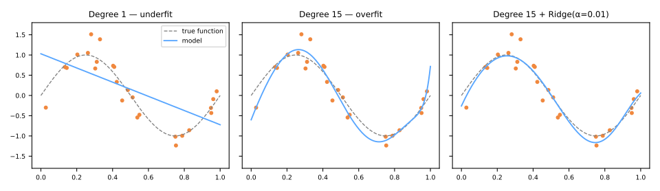
Degree 1 underfits: too rigid. Degree 15 overfits: 16 parameters chase 25 noisy points. Right: the same 16 parameters plus a Ridge penalty, and the curve relaxes back to the signal.
Underfitting and overfitting, measured
100 points of \(y = 0.5x^2 + x + 2\), noise with standard deviation 3; five-fold cross-validation.
| degree | train RMSE | validation RMSE (mean) | spread across folds |
|---|---|---|---|
| 1 | 3.22 | 3.26 | 0.19 |
| 2 | 2.64 | 2.75 | 0.33 |
| 30 | 2.46 | 10.43 | 13.46 |
Degree 30, fold by fold: \(3.14 \quad 3.02 \quad 5.51 \quad \mathbf{37.29} \quad 3.20\)
A pocket diagnostic
| too simple (underfitting) | too complex (overfitting) | |
|---|---|---|
| training error | high | low |
| validation error | high, consistently | high on average, occasionally low |
| spread across folds | small | large |
| what to do | more capacity, better features | regularize, more data, less capacity |
"Too complex" depends on how much data you have
A degree-10 polynomial has 11 free parameters.
| training points | 5 | 8 | 10 | 11 | 15 | 30 |
|---|---|---|---|---|---|---|
| train RMSE | 3·10⁻¹⁵ | 1·10⁻¹¹ | 1·10⁻¹¹ | 0.40 | 0.77 | 1.53 |
- Up to 11 points the curve passes through every one: zero training error means nothing was left over.
- From the eleventh point on it has to choose, and the error lifts off the floor.
Regularization: penalize the magnitude
Ridge (L2) · Tikhonov 1943; Hoerl & Kennard 1970
\[ \lVert y - Xw \rVert^2 + \alpha \sum_j w_j^2 \]- shrinks smoothly, never to exactly zero
- spreads weight across correlated features
- closed form: \((X^\top X + \alpha I)^{-1} X^\top y\)
Lasso (L1) · Tibshirani 1996
\[ \lVert y - Xw \rVert^2 + \alpha \sum_j \lvert w_j \rvert \]- lands exactly at zero for weak features
- automatic feature selection
- among correlated features, keeps one arbitrarily
Elastic Net blends both (l1_ratio): a robust default with many correlated features.
Why L1 zeroes and L2 does not
Write the penalty as a budget: minimize the error subject to \(\sum |w_j| \le t\) (lasso) or \(\sum w_j^2 \le t^2\) (ridge).
- The error contours are ellipses centered on the OLS solution.
- The solution is where the growing ellipse first touches the region.
Simulator: circle versus diamond
Drag the OLS optimum around and count how often each region is touched on an axis.
The one-dimensional case, in closed form
one feature, \(\sum_i x_i^2 = 1\), \(\alpha = 1\)
| \(\hat{w}\) (OLS) | ridge | lasso |
|---|---|---|
| 2.00 | 1.000 | 1.500 |
| 1.00 | 0.500 | 0.500 |
| 0.60 | 0.300 | 0.100 |
| 0.50 | 0.250 | 0 |
| 0.20 | 0.100 | 0 |
Watching the path
Eight features: three with real signal, three pure noise, two near-copies (\(c_1, c_2\), both truly 2). Predict. As \(\alpha\) grows, which coefficients does lasso drop first?
What the path shows
| α | lasso: non-zero | ridge: non-zero |
|---|---|---|
| 0.05 | 8 / 8 | 8 / 8 |
| 0.2 | 7 / 8 | 8 / 8 |
| 0.6 | 6 / 8 | 8 / 8 |
| 2.0 | 5 / 8 | 8 / 8 |
Lasso removes the noise features first; ridge keeps all eight, small.
The correlated pair at \(\alpha = 2\):
lasso (1.89, 0.98): starts to pick one, almost arbitrarily.
ridge (1.02, 0.97): splits the weight evenly.
Ridge also fixes the numerics
two nearly identical columns
condition number of \(X^\top X\): \(7.2\times10^{7}\)
OLS: \((1.000, -0.000)\), an arbitrary split
\(\alpha = 0.01\) on the diagonal
condition number: \(6\times10^{3}\)
answer: \((0.500, 0.500)\), the sum preserved
The knob α
- \(\alpha \to 0\): plain OLS, no brake.
- \(\alpha \to \infty\): every coefficient crushed to ~0, the model predicts the mean.
- The right \(\alpha\) is not known in advance: choose it by cross-validation (
RidgeCV,LassoCV, a grid search).
Summary
- \(w \leftarrow w - \eta\nabla J\); for squared error, \(\nabla J = -\frac{2}{n}X^\top e\), a residual-weighted sum.
- Scale the features: a round bowl instead of a narrow valley.
- \(\eta\) too large diverges; mini-batch is the default.
- Overfitting = low training error, unpredictable validation error.
- Ridge divides, lasso subtracts and clips; choose \(\alpha\) by cross-validation.
Gradient descent, in practice
- Open the handout notebook on Colab (in Portuguese).
- A one-variable slope; the learning rate pushed until it breaks.
- The three points of one step, by hand, checked number by number.
- The loss landscape with and without centering; 20k California houses with and without standardization; mini-batch.