Hierarchical Clustering
In Clustering, k-means needed the number of clusters before it started and returned one flat partition. Hierarchical clustering answers a different question: instead of "split these points into k groups", it builds the whole family of groupings at once, nested inside each other, as a tree. Two animals join, then that pair joins a third, small groups join into larger ones, and at the top everything is one group. The tree is called a dendrogram, and the number of clusters is chosen afterwards, by deciding at what height to cut it.
This is the oldest way of organizing living things (kingdoms, classes, orders, families, species), and it is still what biologists, librarians and marketing teams want when one level of detail is not enough. This lesson builds the tree by hand on five points, reads it, cuts it, measures how the choice of linkage changes what it finds, checks how faithfully it keeps the original distances, and ends with a lab that rebuilds a zoological taxonomy from 16 yes/no questions about 101 animals.
Every claim below is measured, not asserted: each figure is produced by a short Python script that sits next to this page, and the code blocks reproduce the numbers quoted in the text.
The lesson follows one pipeline in four stages, drawn below: 1. build the tree, merging the closest pair again and again, by hand, with four linkages; 2. read and cut, what the dendrogram says and how a cut turns it into groups; 3. choose and check, which linkage, where to cut and how faithfully the tree keeps the distances; 4. in practice, other distances, the cost, and when a tree beats k-means or density-based clustering. Each stage links to its section, and in the slides a strip at the bottom shows which stage you are in.
- Build the treemerge the closest pair; four linkages by hand
- Read and cutthe dendrogram, the matrix Z, the cut
- Choose and checklinkage behaviors, where to cut, cophenetic correlation
- In practiceother distances, cost, against k-means and density-based clustering
Slides
Click the slides and use the ← → arrows to navigate; F goes full screen and Esc shows every slide. Open the slides in a new tab
The idea: merge the two closest groups, repeat
Stage 1. Agglomerative hierarchical clustering is four lines:
- start with \(n\) clusters, one per point;
- find the two clusters that are closest to each other;
- merge them into one, and record the distance at which they merged (the merge height);
- repeat from step 2 until a single cluster is left.
After \(n-1\) merges the history of the merges is the tree. Nothing is random and nothing is iterated to convergence: the same data always gives the same tree (up to ties). The divisive alternative runs the other way — start with one cluster and split it recursively, for example with 2-means at each step — but it is much less common, and everything below is agglomerative.
Step 2 hides the only real decision. Distances between points are given; the distance between two clusters has to be defined. That definition is the linkage:
| linkage | distance between clusters \(P\) and \(Q\) | tends to produce |
|---|---|---|
| single | the closest pair: \(\min_{p \in P,\, q \in Q} d(p, q)\) | chains; follows thin shapes; one outlier bridge merges two groups |
| complete | the farthest pair: \(\max_{p,q} d(p, q)\) | compact groups of similar diameter |
| average (UPGMA) | the mean of all \(\lvert P \rvert \cdot \lvert Q \rvert\) pairwise distances | a compromise between the two |
| Ward | how much the merge increases the within-cluster sum of squares | round groups of similar size, like k-means |
Ward (1963) is the one that connects to the previous lesson. The within-cluster sum of squares is the k-means inertia, and Ward merges the pair of clusters whose union raises it the least:
where \(\mu_P\) and \(\mu_Q\) are the two centroids. k-means minimizes inertia for one fixed \(k\), by iteration; Ward grows it as slowly as it can, one greedy merge at a time.
Build a tree yourself before the worked example. Press merge next a few times on the three blobs and watch each merge add one bar to the dendrogram, then merge all and drag the red cut line up and down. Switch the linkage on the chain and on the two moons, and look for the biggest jump in merge height before you cut.
Single linkage follows each moon but lets the bridge glue the two groups together, and its tree has no clear jump; complete, average and Ward keep the groups compact, so they separate the two blobs of the chain and cut the moons across. Wherever the merge heights jump, a cut inside the jump gives a partition the data support.
Worked by hand: five points, four trees
Five points on a line. The gaps between neighbors grow by one — 3, 4, 5, 6 — which is exactly the kind of data on which the linkages disagree.
| point | A | B | C | D | E |
|---|---|---|---|---|---|
| position | 0 | 3 | 7 | 12 | 18 |
The distance matrix (in 1-D, the distance is just the difference):
| A | B | C | D | E | |
|---|---|---|---|---|---|
| A | 0 | 3 | 7 | 12 | 18 |
| B | 3 | 0 | 4 | 9 | 15 |
| C | 7 | 4 | 0 | 5 | 11 |
| D | 12 | 9 | 5 | 0 | 6 |
| E | 18 | 15 | 11 | 6 | 0 |
Merge 1 is the same for every linkage. Between single points every definition gives the plain distance, so all four merge the closest pair, A and B, at height 3. Now the matrix shrinks to 4 × 4, and the linkages start to differ in how they fill the new row, the distance from \(\{A,B\}\) to everything else:
| distance from {A, B} to | single = min | complete = max | average = mean |
|---|---|---|---|
| C | min(7, 4) = 4 | max(7, 4) = 7 | (7 + 4) / 2 = 5.5 |
| D | min(12, 9) = 9 | max(12, 9) = 12 | (12 + 9) / 2 = 10.5 |
| E | min(18, 15) = 15 | max(18, 15) = 18 | (18 + 15) / 2 = 16.5 |
The rest of the matrix does not change: C–D = 5, C–E = 11, D–E = 6. Merge 2 already splits the linkages. For single linkage the smallest entry is now 4, so C joins {A, B}. For complete and average the new row is larger (7 and 5.5), the smallest entry is C–D = 5, and C pairs with D instead. Continue the same way to the end:
Single linkage — always the smallest gap between the groups, so the chain just grows:
| merge | clusters before | smallest distance between clusters | merges | height |
|---|---|---|---|---|
| 1 | A · B · C · D · E | A–B = 3 | A + B | 3 |
| 2 | AB · C · D · E | AB–C = min(7, 4) = 4 | AB + C | 4 |
| 3 | ABC · D · E | ABC–D = min(12, 9, 5) = 5 | ABC + D | 5 |
| 4 | ABCD · E | ABCD–E = min(18, 15, 11, 6) = 6 | ABCD + E | 6 |
Complete linkage — the largest distance between the groups decides:
| merge | clusters before | candidates | merges | height |
|---|---|---|---|---|
| 2 | AB · C · D · E | AB–C 7, AB–D 12, AB–E 18, C–D 5, C–E 11, D–E 6 | C + D | 5 |
| 3 | AB · CD · E | AB–CD = max(7, 12, 4, 9) = 12; CD–E = max(11, 6) = 11; AB–E 18 | CD + E | 11 |
| 4 | AB · CDE | max of the six A/B-to-C/D/E distances = 18 | AB + CDE | 18 |
Average linkage — the mean of all cross distances:
| merge | clusters before | candidates | merges | height |
|---|---|---|---|---|
| 2 | AB · C · D · E | AB–C 5.5, AB–D 10.5, AB–E 16.5, C–D 5, C–E 11, D–E 6 | C + D | 5 |
| 3 | AB · CD · E | AB–CD = (7 + 12 + 4 + 9) / 4 = 8; CD–E = (11 + 6) / 2 = 8.5; AB–E 16.5 | AB + CD | 8 |
| 4 | ABCD · E | (18 + 15 + 11 + 6) / 4 = 12.5 | ABCD + E | 12.5 |
Merge 3 is where average and complete part ways: 8 against 8.5 is close, and average prefers to join the two pairs, while complete sees the 12 between A and D and prefers to bring E into {C, D}.
Ward works with the cost \(\Delta\), the increase in the sum of squares. For two single points it is half the squared distance (A + B: \(\tfrac{1 \cdot 1}{2}\, 3^2 = 4.5\)); in general it needs the sizes and the centroids:
| merge | clusters before (centroid) | cheapest candidates, \(\Delta\) | merges | \(\Delta\) | height \(\sqrt{2\Delta}\) |
|---|---|---|---|---|---|
| 1 | five singletons | A+B 4.5 · B+C 8 · C+D 12.5 | A + B | 4.5 | 3 |
| 2 | AB (1.5) · C · D · E | C+D 12.5 · D+E 18 · AB+C \(\tfrac{2}{3}(7-1.5)^2 = 20.17\) | C + D | 12.5 | 5 |
| 3 | AB (1.5) · CD (9.5) · E | CD+E \(\tfrac{2}{3}(18-9.5)^2 = 48.17\) · AB+CD \(1 \cdot 8^2 = 64\) · AB+E 181.5 | CD + E | 48.17 | 9.81 |
| 4 | AB (1.5) · CDE (12.33) | AB+CDE \(\tfrac{6}{5}(12.33-1.5)^2 = 140.83\) | AB + CDE | 140.83 | 16.78 |
Two checks you can do with a calculator. The four costs add up to 4.5 + 12.5 + 48.17 + 140.83 = 206, which is the sum of squares of the five points around their mean 8 — the inertia of "one cluster", as it must be, since every merge adds exactly its \(\Delta\). And the last column: libraries report \(\sqrt{2\Delta}\) as the Ward height, so that a merge of two single points sits at their ordinary distance (\(\sqrt{2 \cdot 4.5} = 3\)).
All four update rules above are special cases of one formula, due to Lance & Williams (1967): the distance from a cluster \(K\) to a merged cluster \(I \cup J\) is \(\alpha_I d(K, I) + \alpha_J d(K, J) + \beta\, d(I, J) + \gamma\, |d(K, I) - d(K, J)|\), with a different choice of the four coefficients for each linkage (single: \(\alpha = \tfrac12, \beta = 0, \gamma = -\tfrac12\), which gives the minimum). This is why the algorithm only ever needs the distance matrix, never the points themselves — except for Ward, whose formula is exact only for squared Euclidean distances.
SciPy confirms the four hand computations:
import numpy as np
from scipy.cluster.hierarchy import linkage
from scipy.spatial.distance import pdist, squareform

X = np.array([[0], [3], [7], [12], [18]])        # A, B, C, D, E on a line
names = list('ABCDE')
print(squareform(pdist(X)).astype(int))          # the distance matrix

def merges(Z):
    """Translate a linkage matrix into the sequence of merged groups."""
    groups = list(names)
    steps = []
    for a, b, height, size in Z:
        groups.append(''.join(sorted(groups[int(a)] + groups[int(b)])))
        steps.append(f"{groups[-1]} at {height:.2f}")
    return ' -> '.join(steps)

for method in ['single', 'complete', 'average', 'ward']:
    print(f"{method:8s}", merges(linkage(X, method)))
[[ 0  3  7 12 18]
 [ 3  0  4  9 15]
 [ 7  4  0  5 11]
 [12  9  5  0  6]
 [18 15 11  6  0]]
single   AB at 3.00 -> ABC at 4.00 -> ABCD at 5.00 -> ABCDE at 6.00
complete AB at 3.00 -> CD at 5.00 -> CDE at 11.00 -> ABCDE at 18.00
average  AB at 3.00 -> CD at 5.00 -> ABCD at 8.00 -> ABCDE at 12.50
ward     AB at 3.00 -> CD at 5.00 -> CDE at 9.81 -> ABCDE at 16.78
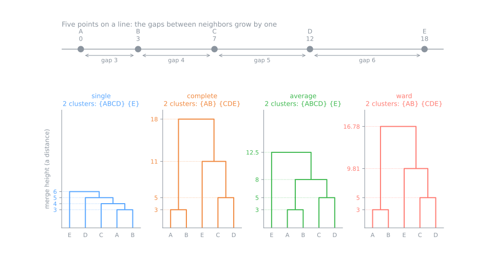
One distance matrix, three different trees (complete and Ward share a shape, with different heights). The disagreement is not a detail: asked for two clusters, single and average isolate E, while complete and Ward cut between B and C. Single linkage sees a chain in which every gap is only one unit larger than the previous one, and finds no reason to break it anywhere but at the last gap. Complete and Ward compare whole groups and see two groups, {A, B} near 1.5 and {C, D, E} near 12.3. Neither is wrong; they are answers to different definitions of "a cluster".
Reading a dendrogram
Stage 2. A dendrogram has one leaf per point along the bottom and one horizontal bar per merge. The rules for reading it:
- The y-axis is a distance. The height of a bar is the linkage distance at which its two branches merged. Two points are as similar as the height of the lowest bar that connects them: in the complete tree, A and B join at 3, but A and E only at 18. That height is called the cophenetic distance between the two points.
- Long vertical lines are the interesting part. A branch that survives a long way up before merging is a group that stays far from everything else. In the complete tree, {C, D, E} forms at 11 and waits until 18 to join {A, B}.
- The left-to-right order carries almost no information. Each bar can be flipped without changing the tree, so 5 leaves have \(2^4 = 16\) equivalent drawings. In the complete tree E is drawn right next to B, although they are the two points that end up farthest apart (18). Never read similarity from neighboring leaves; read it from the height where they meet.
The tree is stored in a linkage matrix Z with \(n - 1\) rows, one per merge, in the order the merges happened:
Column by column:
| column | meaning | complete tree |
|---|---|---|
| 0 and 1 | the two clusters merged. Ids 0 to \(n-1\) are the original points; the cluster created by row \(i\) gets id \(n + i\) | row 0 merges points 0 and 1 (A, B) into cluster 5; row 1 merges 2 and 3 (C, D) into cluster 6; row 2 merges point 4 (E) with cluster 6; row 3 merges clusters 5 and 7 |
| 2 | the merge height | 3, 5, 11, 18 — the heights of the hand table |
| 3 | how many original points the new cluster contains | 2, 2, 3, 5 |
dendrogram draws it (the figure above is four calls of it), and with no_plot=True it returns the left-to-right leaf order without drawing:
import matplotlib.pyplot as plt
from scipy.cluster.hierarchy import dendrogram

dendrogram(Z, labels=names)
plt.ylabel('merge height')
plt.show()
print(dendrogram(Z, labels=names, no_plot=True)['ivl'])
Cutting the tree
A horizontal line drawn across the dendrogram at height \(t\) cuts some vertical lines; each piece hanging below the line is one cluster. SciPy's fcluster does it two ways: at a given height (criterion='distance') or for a requested number of clusters (criterion='maxclust'):
from scipy.cluster.hierarchy import fcluster

for t in [4, 8, 12, 20]:
    print(f"cut at height {t:2d}:", fcluster(Z, t, criterion='distance'))
for k in [2, 3]:
    print(f"ask for {k} clusters: ", fcluster(Z, k, criterion='maxclust'))
cut at height  4: [1 1 2 3 4]
cut at height  8: [1 1 2 2 3]
cut at height 12: [1 1 2 2 2]
cut at height 20: [1 1 1 1 1]
ask for 2 clusters:  [1 1 2 2 2]
ask for 3 clusters:  [1 1 2 2 3]
Read against the complete tree: a line at 4 is above the A–B merge (3) only, so A and B share a label and the other three are alone, 4 clusters. At 8 it also passes above C–D (5): {A, B}, {C, D}, {E}. At 12 it passes above 11 as well: {A, B} and {C, D, E}. Any cut between 11 and 18 gives the same two clusters. That range of heights, 7 units wide, is what makes the two-cluster answer stable here; the next section turns that into a way of choosing \(k\).
scikit-learn wraps the same algorithm in AgglomerativeClustering, with the usual fit_predict interface. Give it n_clusters, or set n_clusters=None and give it a height as distance_threshold:
from sklearn.cluster import AgglomerativeClustering

for method in ['single', 'complete', 'average', 'ward']:
    agg = AgglomerativeClustering(n_clusters=2, linkage=method, compute_distances=True).fit(X)
    print(f"{method:8s} labels {agg.labels_}  merge heights {agg.distances_.round(2)}")

agg = AgglomerativeClustering(n_clusters=None, distance_threshold=8, linkage='complete').fit(X)
print(f"complete, cut at 8: {agg.n_clusters_} clusters, labels {agg.labels_}")
single   labels [0 0 0 0 1]  merge heights [3. 4. 5. 6.]
complete labels [1 1 0 0 0]  merge heights [ 3.  5. 11. 18.]
average  labels [0 0 0 0 1]  merge heights [ 3.   5.   8.  12.5]
ward     labels [1 1 0 0 0]  merge heights [ 3.    5.    9.81 16.78]
complete, cut at 8: 3 clusters, labels [1 1 0 0 2]
The merge heights are the ones in the hand tables, Ward included (scikit-learn uses the same \(\sqrt{2\Delta}\) scale). The label numbers differ from SciPy's (0/1 instead of 1/2, in another order), which does not matter: a partition is the grouping, not the names of the groups.
AgglomerativeClustering has no predict method. A tree is built from the points it was given; a new point has no place in it until you rebuild the tree, or until you assign it with some other rule (for example, to the cluster of its nearest neighbor or centroid, as in the section on cost).
One property follows from the construction and is worth stating: cuts of the same tree are nested. The 3-cluster cut is the 2-cluster cut with one cluster split in two; nothing ever moves between branches. Two k-means runs with \(k = 3\) and \(k = 4\) have no such obligation, and the lab measures how much they disagree.
Linkage behaviors, measured
Stage 3. The five points showed that the linkages can disagree. On real shapes the disagreement follows a pattern. Four 2-D datasets with known groups, 300 points each, and every method is told the true number of clusters, so the only difference is the linkage. The score is the adjusted Rand index (ARI) from Clustering: 1 for a partition identical to the true groups, around 0 for one no better than chance.
from sklearn.datasets import make_blobs, make_moons
from sklearn.metrics import adjusted_rand_score
import pandas as pd

rng = np.random.default_rng(0)
blobs = make_blobs(n_samples=300, centers=3, cluster_std=1.0, random_state=1)
a, b = rng.normal([0, 0], 0.7, (140, 2)), rng.normal([6, 0], 0.7, (140, 2))
t = np.linspace(1.0, 5.0, 20)                                     # a thin line of 20 points
bridge = (np.vstack([a, b, np.c_[t, rng.normal(0, 0.05, 20)]]),
          np.r_[np.zeros(140), np.ones(140), (t > 3).astype(int)])
moons = make_moons(n_samples=300, noise=0.06, random_state=0)
rng = np.random.default_rng(0)
strips = (np.vstack([np.c_[rng.uniform(0, 8, 100), rng.normal(1.5 * j, 0.12, 100)] for j in range(3)]),
          np.repeat([0, 1, 2], 100))

table = {}
for name, (Xd, yd) in {'blobs': blobs, 'blobs + bridge': bridge,
                       'moons': moons, 'parallel strips': strips}.items():
    k = len(np.unique(yd))
    table[name] = {m: adjusted_rand_score(yd, AgglomerativeClustering(n_clusters=k, linkage=m).fit_predict(Xd))
                   for m in ['single', 'complete', 'average', 'ward']}
print(pd.DataFrame(table).T.round(2))
                 single  complete  average  ward
blobs              0.57      0.98     0.98  0.98
blobs + bridge     0.00      0.91     0.99  0.96
moons              1.00      0.20     0.43  0.30
parallel strips    1.00      0.12     0.19  0.22
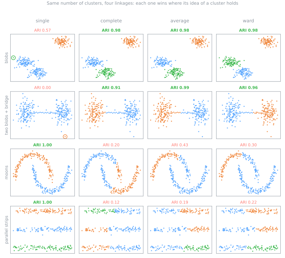
The table splits cleanly into two camps:
- Single linkage wins exactly where the others lose. On the moons and on the parallel strips it scores 1.00: each shape is a chain of close neighbors, and single linkage only ever asks "is there some short hop between these groups?". The same question is its weakness. On the blobs it scores 0.57: it keeps one far-away point as a cluster of its own (circled) and lumps two blobs together. With two blobs joined by a thin bridge of 20 points it scores 0.00: the bridge offers a chain of short hops, so the two blobs merge early, and the last merge left is some stray point. This is chaining. Single linkage is also the minimum spanning tree in disguise (Gower & Ross, 1969): cutting the tree at height \(t\) is the same as deleting every edge longer than \(t\) from the minimum spanning tree.
- Complete, average and Ward ask how far apart the groups are as a whole, so a bridge of a few points cannot pull two blobs together (0.91 to 0.99). But they all prefer compact groups, so they cut the moons and the strips across (0.12 to 0.43), exactly as k-means does. Ward is the most k-means-like; complete is the most sensitive to a single far point, since one outlier sets the maximum; average sits between them.
The practical rule: Ward (the default in scikit-learn) or average for compact groups; single when you expect thin, connected shapes and the groups are well separated; and always look at the tree before trusting any of them.
Choosing where to cut
A tree has \(n - 1\) possible cuts, so something has to choose. Take 400 points in four blobs that come in two pairs: two scales of structure in one dataset.
from sklearn.metrics import silhouette_score

X4, y4 = make_blobs(n_samples=400, centers=[[0, 0], [0, 3.5], [9, 6], [12, 6]],
                    cluster_std=0.8, random_state=0)
Z4 = linkage(X4, 'ward')
h = Z4[::-1, 2]                  # heights from the top: h[0] merges 2 -> 1 clusters, h[1] 3 -> 2, ...
print('top merge heights:', h[:6].round(1))
for k in range(2, 8):
    labels = fcluster(Z4, k, criterion='maxclust')
    print(f"k={k}: any cut between {h[k-1]:5.1f} and {h[k-2]:5.1f} (gap {h[k-2] - h[k-1]:5.1f})"
          f"  silhouette {silhouette_score(X4, labels):.3f}")
top merge heights: [159.2  32.3  30.3   9.7   9.2   8.9]
k=2: any cut between  32.3 and 159.2 (gap 126.9)  silhouette 0.787
k=3: any cut between  30.3 and  32.3 (gap   2.1)  silhouette 0.664
k=4: any cut between   9.7 and  30.3 (gap  20.6)  silhouette 0.545
k=5: any cut between   9.2 and   9.7 (gap   0.5)  silhouette 0.473
k=6: any cut between   8.9 and   9.2 (gap   0.3)  silhouette 0.393
k=7: any cut between   8.7 and   8.9 (gap   0.2)  silhouette 0.349
The largest gap in merge heights. The \(k\)-cluster partition is what you get for every cut height between the merge that created it and the merge that destroys it. The wider that range, the more the data insist on that \(k\): a tiny gap means a slightly different height, or slightly different data, would give another answer. Here \(k = 2\) survives a range of 126.9 (from 32.3 to 159.2), and \(k = 4\) a range of 20.6; no other \(k\) survives more than 2.1. Two gaps stand out because there are two scales: the pairs are far apart, and inside each pair there are two blobs.
The silhouette of each cut, from Clustering, measured on the same points. It is highest at \(k = 2\) (0.787) and falls steadily: 0.545 at \(k = 4\). It agrees with the biggest gap, and, like every compactness index, it prefers the coarsest well-separated split. It does not see the second scale at all.
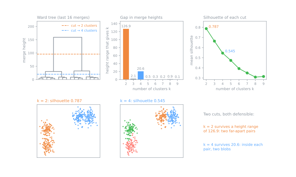
So which is right? Both, and this is the real advantage of a tree: you do not have to choose only one. The two cuts are nested, so you can report two segments at the coarse level and four at the fine level, and they agree with each other. When one number is required, choose with the question in mind (how many groups can someone act on?) and use the gaps and the silhouette to rule out cuts that are not supported by the data, as k = 3 is not here (gap 2.1).
SciPy also offers the inconsistency coefficient, which compares each merge height with the heights of the merges just below it: \((h - \text{mean}) / \text{std}\), computed over the link and its sub-links down to depth d. A merge much higher than the merges it joins is "inconsistent", a natural place to cut, and fcluster(Z, t, criterion='inconsistent') cuts wherever the coefficient exceeds t:
from scipy.cluster.hierarchy import inconsistent

print(inconsistent(Z4, d=2)[-4:].round(2))     # last 4 merges: mean, std, count, coefficient
Each row is one merge: the mean and standard deviation of the heights used (the link itself and the links just below it), how many heights that was, and the coefficient. It is a local measure, and here it shows its limit: with depth 2 the statistics use at most three heights, so the coefficient cannot exceed \(2/\sqrt{3} = 1.15\), and the top three merges all get that maximum. It cannot tell the \(k = 2\) boundary from the \(k = 4\) one, while the gaps can. Use it, if at all, as one more hint.
Cophenetic correlation: how faithful is the tree?
A tree replaces the \(n(n-1)/2\) pairwise distances by \(n - 1\) merge heights. Each pair of points gets a new distance, the cophenetic distance (the height at which they first join), and the question is how much of the original geometry survives. Sokal & Rohlf (1962) proposed the obvious measure: the correlation between the original distances and the cophenetic ones, the cophenetic correlation.
By hand, for the single-linkage tree of the five points. List the 10 pairs in the order AB, AC, AD, AE, BC, BD, BE, CD, CE, DE:
| AB | AC | AD | AE | BC | BD | BE | CD | CE | DE | mean | |
|---|---|---|---|---|---|---|---|---|---|---|---|
| original \(d\) | 3 | 7 | 12 | 18 | 4 | 9 | 15 | 5 | 11 | 6 | 9 |
| cophenetic \(c\) | 3 | 4 | 5 | 6 | 4 | 5 | 6 | 5 | 6 | 6 | 5 |
Centered, the products \((d - 9)(c - 5)\) add up to 33, the squares \((d - 9)^2\) to 220 and \((c - 5)^2\) to 10, so the correlation is \(33 / \sqrt{220 \times 10} = 0.704\). SciPy's cophenet returns the same number, and the other three trees:
from scipy.cluster.hierarchy import cophenet

dist = pdist(X)
for method in ['single', 'complete', 'average', 'ward']:
    c, coph = cophenet(linkage(X, method), dist)
    print(f"{method:8s} cophenetic correlation {c:.3f}   cophenetic distances {coph.round(1)}")
single   cophenetic correlation 0.704   cophenetic distances [3. 4. 5. 6. 4. 5. 6. 5. 6. 6.]
complete cophenetic correlation 0.565   cophenetic distances [ 3. 18. 18. 18. 18. 18. 18.  5. 11. 11.]
average  cophenetic correlation 0.691   cophenetic distances [ 3.   8.   8.  12.5  8.   8.  12.5  5.  12.5 12.5]
ward     cophenetic correlation 0.561   cophenetic distances [ 3.  16.8 16.8 16.8 16.8 16.8 16.8  5.   9.8  9.8]
Single linkage keeps the distances best here (0.704), even though its tree is a chain, and complete and Ward, whose two-cluster cut looked the most natural, keep them worst (0.565 and 0.561): they push every A/B-to-C/D/E pair to one big height, 18 or 16.78, erasing the difference between B–C (4) and A–E (18). The same comparison on the four blobs of the previous section:
d4 = pdist(X4)
for method in ['single', 'complete', 'average', 'ward']:
    Zm = linkage(X4, method)
    print(f"{method:8s} cophenetic correlation {cophenet(Zm, d4)[0]:.3f}"
          f"   ARI at k=4 {adjusted_rand_score(y4, fcluster(Zm, 4, criterion='maxclust')):.3f}")
single   cophenetic correlation 0.944   ARI at k=4 0.496
complete cophenetic correlation 0.947   ARI at k=4 0.954
average  cophenetic correlation 0.953   ARI at k=4 0.856
ward     cophenetic correlation 0.952   ARI at k=4 0.892
All four trees keep the distances almost equally well (0.944 to 0.953), and yet their four-cluster cuts range from ARI 0.496 (single, which chains two blobs together) to 0.954 (complete). This is the point to remember. Cophenetic correlation measures how faithfully the tree represents the distances, not how good the clusters are. Average linkage often scores highest, because the mean of the cross distances is a natural summary of them. Use the cophenetic correlation to compare linkages when the tree itself is the product — a taxonomy, the order of a heat map — and the cluster checks (gaps, silhouette, and a look at the data) for the clusters.
Beyond Euclidean distance
Stage 4. Nothing in the algorithm needs Euclidean distance: single, complete and average linkage work with any dissimilarity. That opens two important cases.
Profiles: correlation distance. Four customers, six months of spending. Two of them grow steadily, two spend mostly in one month; one of each pair spends five times more than the other:
P = np.array([[10, 12, 14, 16, 18, 20],           # small, steady growth
              [50, 60, 70, 80, 90, 100],          # large, steady growth
              [12, 10, 11, 25, 11, 10],           # small, one peak month
              [55, 50, 52, 110, 50, 52]], float)  # large, one peak month
for metric in ['euclidean', 'correlation']:
    Zp = linkage(P, 'average', metric=metric)
    print(f"{metric:11s} clusters {fcluster(Zp, 2, criterion='maxclust')}   distances {pdist(P, metric).round(2)}")
euclidean   clusters [1 2 1 2]   distances [150.73  15.72 125.69 157.45  72.48 125.06]
correlation clusters [1 1 2 2]   distances [0.   0.94 0.9  0.94 0.9  0.  ]
Euclidean distance groups the customers by how much they spend (small with small, large with large); correlation distance, \(1 - r\), groups them by the shape of their spending (growers with growers, peaks with peaks), because a profile and the same profile multiplied by five have correlation 1 and distance 0. Which one is right depends on the question, and no index computed on the data can tell you. Gene-expression analysis uses correlation distance for this reason: two genes that rise and fall together across samples are related, whatever their baseline level.
Documents: cosine distance. In Text Representation, a document becomes a vector of word counts. A document and the same document written ten times longer point in the same direction but are far apart in Euclidean distance:
docs = np.array([[2, 1, 0, 0],       # a short text about topic 1
                 [20, 10, 0, 0],     # a long text, same words, same proportions
                 [0, 0, 3, 1]])      # a short text about topic 2
for metric in ['euclidean', 'cosine']:
    print(f"{metric:9s}", squareform(pdist(docs, metric)).round(2)[0])
Measured from the first document, Euclidean distance says the text on the other topic is closer (3.87) than the same text written longer (20.12); cosine distance says the opposite (1.0 against 0.0). For text, cosine is the default. In scikit-learn, AgglomerativeClustering(metric='cosine', linkage='average'), or metric='precomputed' with any matrix you computed yourself. Ward is the exception: its cost is defined through centroids and squared Euclidean distances, and scikit-learn refuses any other metric with linkage='ward'.
Connectivity constraints. AgglomerativeClustering also accepts a connectivity matrix, for example kneighbors_graph(X, n_neighbors=10), and then only merges clusters that are neighbors in that graph. Two groups that happen to be close in space but are not connected through the data cannot merge, which makes even Ward follow thin, curved structures; it is the standard way to segment an image into regions of adjacent pixels, or a map into contiguous areas. Because only neighboring pairs are ever compared, it is also much faster on large data.
Cost: why it does not scale, and what to do
Every standard agglomerative algorithm starts from the full matrix of pairwise distances. That is \(n(n-1)/2\) numbers:
for n in [1_000, 10_000, 100_000, 1_000_000]:
    print(f"{n:>9,} rows: {n * (n - 1) // 2:>15,} distances = {n * (n - 1) / 2 * 8 / 1e9:9,.3f} GB")
    1,000 rows:         499,500 distances =     0.004 GB
   10,000 rows:      49,995,000 distances =     0.400 GB
  100,000 rows:   4,999,950,000 distances =    40.000 GB
1,000,000 rows: 499,999,500,000 distances = 3,999.996 GB
Time is worse than memory. The naive algorithm (search the whole matrix for the minimum, merge, repeat) is \(O(n^3)\); the algorithms SciPy and scikit-learn actually use, described by Müllner (2011), bring the four linkages of this lesson down to \(O(n^2)\) — a minimum spanning tree for single linkage, and the nearest-neighbor chain for complete, average and Ward. \(O(n^2)\) is still quadratic. Measured on 5-D blobs:
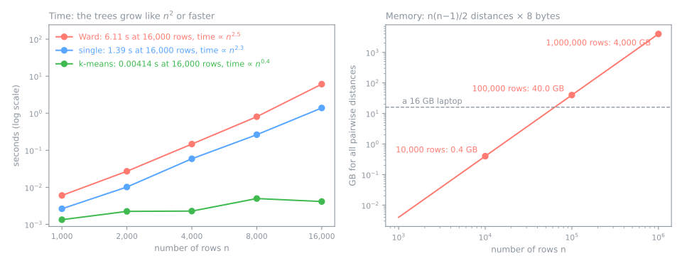
On the machine that drew the figure, each doubling of \(n\) multiplied the time by about 5.7, and 16,000 rows took 6.11 s with Ward; k-means on the same rows took 0.004 s. (Timings change from machine to machine; the exponents are what matter.) Extrapolate one more factor of six (to 100,000 rows) and the distances alone need 40 GB, more than most laptops have. Hierarchical clustering is a method for hundreds to tens of thousands of rows. For more:
- Sample, then assign. Build the tree on a random sample, cut it, and give every other point the cluster of the nearest centroid (or nearest sampled neighbor). If the clusters are large enough to appear in the sample, little is lost:
Xbig, ybig = make_blobs(n_samples=100_000, centers=5, n_features=5, cluster_std=1.5, random_state=0)
rng = np.random.default_rng(0)
idx = rng.choice(len(Xbig), 2_000, replace=False)                 # a 2% sample
lab_sample = fcluster(linkage(Xbig[idx], 'ward'), 5, criterion='maxclust')
centroids = np.array([Xbig[idx][lab_sample == c].mean(axis=0) for c in range(1, 6)])
lab_all = ((Xbig[:, None, :] - centroids[None]) ** 2).sum(axis=2).argmin(axis=1)
print(f"tree on {len(idx):,} rows, all {len(Xbig):,} assigned: ARI {adjusted_rand_score(ybig, lab_all):.3f}")
The tree on 2,000 rows takes a fraction of a second, and its five clusters, extended to all 100,000 rows, match the true groups with ARI 0.993. What you lose is the fine structure: a group of 30 points in 100,000 would have about 0.6 representatives in the sample.
- Connectivity constraints (above) replace the full matrix by a sparse neighbor graph.
- HDBSCAN, from Clustering, is itself a hierarchical method: it builds a single-linkage tree on a density-adjusted distance and keeps the branches that persist longest. With a spatial index it does not need the full distance matrix, so it reaches data sizes far beyond what a linkage can handle, and it marks noise, which no linkage does.
Hierarchical vs k-means vs DBSCAN
| hierarchical (agglomerative) | k-means | DBSCAN / HDBSCAN | |
|---|---|---|---|
| a cluster is | a branch of the merge tree | the points nearest one centroid | a dense region |
| decided before fitting | linkage and distance | \(k\) | eps, min_samples (HDBSCAN: min_cluster_size) |
| decided after fitting | \(k\) or the cut height, from the tree | — | — |
| output | a nested family of partitions | one partition | one partition plus noise (−1) |
| shapes found | depends on the linkage: single follows chains, Ward finds round groups | convex, similar sizes | any shape |
| outliers | kept, as tiny clusters or chained in | forced into a cluster | labeled noise |
| any distance? | yes, except Ward | Euclidean only | yes |
| new points | no predict: rebuild or assign to nearest | predict | no predict in scikit-learn |
| cost | \(O(n^2)\) memory, \(O(n^2)\) time or worse | about linear in \(n\) | about \(n \log n\) with an index |
| same result every run | yes | depends on the initialization | yes |
Applications
Taxonomies. Whenever the product is a tree rather than a partition: species from traits or DNA (the origin of the method, Sokal & Rohlf's numerical taxonomy), product catalogs, the topics of a document collection organized into themes and sub-themes. The lab rebuilds the zoologists' classes of 101 animals this way.
Gene-expression heat maps. A table of genes × samples is unreadable in its original order. Cluster the genes (rows) and the samples (columns) separately, with correlation distance, and redraw the table with both in dendrogram leaf order. Genes that go up and down together end up side by side, and so do samples with the same profile. This is the "clustered heat map" of almost every genomics paper (seaborn's clustermap does it in one call; here it is with SciPy and matplotlib only):
from scipy.cluster.hierarchy import leaves_list

rng = np.random.default_rng(3)
E = rng.normal(size=(40, 12))                                         # any genes x samples table
Ez = (E - E.mean(axis=1, keepdims=True)) / E.std(axis=1, keepdims=True)   # z-score each gene
rows = leaves_list(linkage(Ez, 'average', metric='correlation'))      # gene order
cols = leaves_list(linkage(Ez.T, 'average', metric='correlation'))    # sample order
plt.imshow(Ez[rows][:, cols], aspect='auto', cmap='RdBu_r')
plt.show()
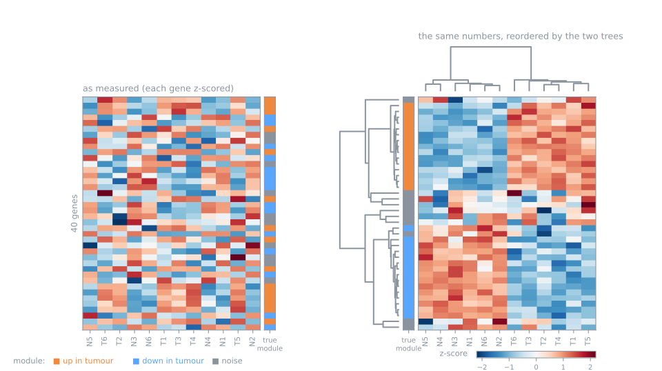
The figure uses a synthetic table with a known answer: 15 genes that go up in tumours, 15 that go down, and 10 of noise, each gene with its own baseline level, rows and columns shuffled. Nothing is visible on the left. On the right, with no information but the numbers, the column tree splits the six tumour samples from the six normal ones at its top merge, and the true-module strip beside the rows turns into solid blocks: the tree has recovered both factors of the design.
Segmentation at several granularities. A marketing team rarely knows whether it wants 3 segments or 12. A single tree on the customer table answers both, consistently: the 12 fine segments are subdivisions of the 3 coarse ones, so a campaign designed for a coarse segment still applies to its sub-segments. Separate k-means runs with \(k = 3\) and \(k = 12\) give no such guarantee.
Lab: a tree of 101 animals
The data. The UCI Zoo table (Forsyth, 1990): 101 animals, each described by 15 yes/no questions (does it have hair? feathers? does it lay eggs? produce milk? fly? live in water? …) and the number of legs. It also has the class a zoologist would give — mammal, bird, fish, reptile, amphibian, insect, invertebrate — which we keep sealed until step 8, as in the wine lab of the clustering lesson: every decision (scaling, linkage, cut) is made the way it would be made without an answer key, and the key is then used only to audit those decisions.
The question. Can a tree built from 16 plain features rediscover the zoologists' taxonomy? And what does it show that k-means does not?
We use OpenML copy 42667 of the table because it keeps the animal names (the older copy, OpenML 62, drops them). Every output below is what the code prints; the whole lab runs in a few seconds. To work on it directly, download the lab notebook and open it in Jupyter or Colab (File → Upload notebook).
Step 1 — load and look
import numpy as np
import pandas as pd
from sklearn.datasets import fetch_openml

zoo = fetch_openml(data_id=42667, as_frame=True).frame     # UCI Zoo, with the animal names
animals = zoo['animal'].to_numpy()
kind = zoo['type']                                          # the zoologists' class: sealed until step 8
X = zoo.drop(columns=['animal', 'type'])
for col in X.columns.drop('legs'):
    X[col] = (X[col].astype(str) == 'True').astype(int)    # yes/no -> 1/0
print(X.shape)
pick = [list(animals).index(a) for a in ['bear', 'chicken', 'crab']]
print(X.iloc[pick].set_axis(animals[pick]).T.to_string())
print('legs:', X['legs'].value_counts().sort_index().to_dict())
print('rows identical to an earlier row:', X.duplicated().sum())
(101, 16)
          bear  chicken  crab
hair         1        0     0
feathers     0        1     0
eggs         0        1     1
milk         1        0     0
airborne     0        1     0
aquatic      0        0     1
predator     1        0     1
toothed      1        0     0
backbone     1        1     0
breathes     1        1     0
venomous     0        0     0
fins         0        0     0
legs         4        2     4
tail         0        1     0
domestic     0        1     0
catsize      1        0     0
legs: {0: 23, 2: 27, 4: 38, 5: 1, 6: 10, 8: 2}
rows identical to an earlier row: 42
Sixteen columns: fifteen are 0/1 answers, legs is a count from 0 to 8. Two things to notice before clustering. First, 42 of the 101 rows are exact copies of an earlier row: many animals are indistinguishable by these 16 questions (most fish, for example, answer everything the same way). The tree will merge them at height 0. Second, "frog" appears twice in the table, as two different animals, one of them venomous.
Step 2 — put the columns on the same scale
raw = X.to_numpy(dtype=float)
sq = (raw[:, None, :] - raw[None, :, :]) ** 2               # every pair, every column
share = pd.Series(sq.sum(axis=(0, 1)) / sq.sum(), index=X.columns)
print(share.sort_values(ascending=False).head(3).round(3))

from sklearn.preprocessing import MinMaxScaler

Xs = MinMaxScaler().fit_transform(X)                        # legs / 8; the 0/1 columns stay 0/1
sq = (Xs[:, None, :] - Xs[None, :, :]) ** 2
print('share of legs after scaling:', round(sq[:, :, X.columns.get_loc('legs')].sum() / sq.sum(), 3))
yes_no = X.columns != 'legs'
i, j = pick[1], pick[2]
print(f"chicken vs crab: {(raw[i] != raw[j])[yes_no].sum()} yes/no answers differ, "
      f"legs {raw[i, ~yes_no][0]:.0f} vs {raw[j, ~yes_no][0]:.0f}, "
      f"squared distance {((Xs[i] - Xs[j]) ** 2).sum():.4f}")
legs        0.589
predator    0.036
catsize     0.035
dtype: float64
share of legs after scaling: 0.022
chicken vs crab: 8 yes/no answers differ, legs 2 vs 4, squared distance 8.0625
How to read it:
- Unscaled,
legsis the clustering. Summed over all pairs of animals, 58.9% of the squared Euclidean distance comes from that one column; each of the other fifteen contributes less than 4%. A difference of two legs weighs as much as four yes/no answers. This is the scaling problem of Preprocessing again, in its purest form. - Which scaler?
MinMaxScalermapslegsto [0, 1] (divides by 8) and leaves the 0/1 columns exactly as they are. After it,legscontributes 2.2%, and the squared distance has a plain meaning: the number of yes/no questions on which two animals disagree, plus a small term for legs. The chicken and the crab disagree on 8 questions and differ by two legs, \((2/8)^2 = 0.0625\), total 8.0625.StandardScalerwould divide each column by its own standard deviation instead, which gives a rare answer (venomous, 8 animals) about three times the weight of a common one (hair); there is no zoological reason for that, so we do not.
As the wine lab showed, no clustering index can make this decision for you: an index computed after scaling measures the geometry the scaling created. It is decided by what a distance should mean for these data.
Step 3 — four linkages, and how faithful each tree is
from scipy.cluster.hierarchy import cophenet, linkage
from scipy.spatial.distance import pdist

d = pdist(Xs)                                               # the 5,050 pairwise distances
trees = {m: linkage(Xs, m) for m in ['single', 'complete', 'average', 'ward']}
for m, Z in trees.items():
    print(f"{m:8s} cophenetic correlation {cophenet(Z, d)[0]:.3f}   top merge at {Z[-1, 2]:.2f}")
single   cophenetic correlation 0.867   top merge at 2.00
complete cophenetic correlation 0.885   top merge at 3.68
average  cophenetic correlation 0.905   top merge at 2.75
ward     cophenetic correlation 0.802   top merge at 14.03
Average linkage keeps the original distances best, with a cophenetic correlation of 0.905; complete (0.885) and single (0.867) follow, and Ward is last (0.802). Ward's heights live on another scale (its top merge is at 14.03, against 2.00 to 3.68 for the others, because it measures growth in the sum of squares, not a distance between animals), and its tree compresses many different pairs into a few large heights. Since the product we want is a taxonomy, a tree whose heights can be read as "how different are these animals", we continue with average linkage. This is the use the cophenetic correlation is made for: choosing among trees when the tree itself is the result.
Step 4 — draw the tree
import matplotlib.pyplot as plt
from scipy.cluster.hierarchy import dendrogram

Z = trees['average']
print('merges at height 0 (identical animals):', (Z[:, 2] == 0).sum())
print('last 8 merge heights:', Z[-8:, 2].round(3))
fig, ax = plt.subplots(figsize=(7, 15))
dendrogram(Z, labels=animals, orientation='left', leaf_font_size=7, ax=ax)
ax.set_xlabel('merge height (average distance between the two groups)')
plt.show()
merges at height 0 (identical animals): 42
last 8 merge heights: [1.894 1.917 2.009 2.097 2.258 2.445 2.519 2.752]
The first 42 merges happen at height 0: they are the 42 duplicate rows of step 1, absorbed into their twins before anything else happens. The last eight merges, the ones that shape the top of the tree, climb from 1.894 to 2.752. The plot is tall on purpose (101 names); the annotated version is at step 9. Before reading any further, look at the plot and write down how many groups you would say there are.
Step 5 — choose the cut: gaps and silhouette
from scipy.cluster.hierarchy import fcluster
from sklearn.metrics import silhouette_score

h = Z[::-1, 2]                          # h[0] merges 2 -> 1 clusters, h[1] merges 3 -> 2, ...
rows = []
for k in range(2, 11):
    labels = fcluster(Z, k, criterion='maxclust')
    rows.append({'k': k, 'gap': h[k - 2] - h[k - 1], 'silhouette': silhouette_score(Xs, labels),
                 'sizes': sorted(np.bincount(labels)[1:], reverse=True)})
print(pd.DataFrame(rows).round(3).to_string(index=False))
 k   gap  silhouette                              sizes
 2 0.233       0.325                           [60, 41]
 3 0.074       0.346                       [41, 39, 21]
 4 0.187       0.398                   [41, 21, 21, 18]
 5 0.161       0.389                [41, 21, 21, 17, 1]
 6 0.087       0.403             [41, 21, 21, 10, 7, 1]
 7 0.092       0.405          [41, 21, 14, 10, 7, 7, 1]
 8 0.022       0.383       [35, 21, 14, 10, 7, 7, 6, 1]
 9 0.025       0.380    [35, 21, 13, 10, 7, 7, 6, 1, 1]
10 0.169       0.377 [35, 21, 13, 10, 7, 7, 5, 1, 1, 1]
How to read it:
- Gaps. The widest range of heights belongs to \(k = 2\) (0.233): one branch of 41 animals against the other 60. The next widest are \(k = 4\) (0.187) and \(k = 5\) (0.161). \(k = 3\) and \(k = 8\), \(k = 9\) have narrow ranges and are poorly supported. (\(k = 10\) has a wide range too, 0.169, but it only peels off single animals: sizes 1, 1, 1.)
- Silhouette. It is highest at \(k = 7\) (0.405), but \(k = 4\), 6 and 7 are within 0.007 of each other; the curve is a plateau from 4 to 7, not a peak.
- Sizes. From \(k = 5\) on, one "cluster" is a single animal. That is not necessarily wrong — some animals are genuinely unlike the rest — but it is worth knowing which one.
The instruments do not name one \(k\), and a tree does not force you to pick one. We keep two nested levels: \(k = 4\) as the coarse level (the second-widest gap and a silhouette on the plateau) and \(k = 7\) as the fine level (the best silhouette). Note that we chose them without looking at the zoologists' classes.
Step 6 — what are the clusters? Profile them
hc4 = fcluster(Z, 4, criterion='maxclust')
hc7 = fcluster(Z, 7, criterion='maxclust')
profile = pd.DataFrame(Xs, columns=X.columns).groupby(hc4).mean()
profile.insert(0, 'size', np.bincount(hc4)[1:])
print(profile[['size', 'hair', 'milk', 'feathers', 'backbone', 'fins', 'toothed', 'legs', 'airborne']].round(2).to_string())
for c in range(1, 8):
    members = animals[hc7 == c]
    print(f"k=7 cluster {c} ({len(members):2d}):", ', '.join(members[:6]) + (' ...' if len(members) > 6 else ''))
   size  hair  milk  feathers  backbone  fins  toothed  legs  airborne
1    41  0.95   1.0      0.00       1.0  0.10     0.98  0.42      0.05
2    21  0.00   0.0      0.00       1.0  0.62     1.00  0.12      0.00
3    21  0.00   0.0      0.95       1.0  0.00     0.00  0.26      0.76
4    18  0.22   0.0      0.00       0.0  0.00     0.00  0.59      0.33
k=7 cluster 1 (41): aardvark, antelope, bear, boar, buffalo, calf ...
k=7 cluster 2 ( 7): frog, frog, newt, pitviper, slowworm, toad ...
k=7 cluster 3 (14): bass, carp, catfish, chub, dogfish, haddock ...
k=7 cluster 4 (21): chicken, crow, dove, duck, flamingo, gull ...
k=7 cluster 5 ( 7): clam, crab, crayfish, lobster, octopus, seawasp ...
k=7 cluster 6 (10): flea, gnat, honeybee, housefly, ladybird, moth ...
k=7 cluster 7 ( 1): scorpion
Each number in the profile is the fraction of the cluster that answers "yes" (for legs, the mean number of legs divided by 8). Read as a zoologist would:
- cluster 1 (41): hair 0.95, milk 1.00 — mammals;
- cluster 2 (21): backbone and teeth in all, 62% with fins, no hair, milk or feathers — the cold-blooded vertebrates, fish together with amphibians and reptiles;
- cluster 3 (21): feathers 0.95, airborne 0.76, backbone 1.00 — birds;
- cluster 4 (18): no backbone at all, the most legs (0.59, about 4.7 on average) — the invertebrates.
The \(k = 7\) level splits clusters 2 and 4: fish (14) apart from frogs, newts and snakes (7); sea invertebrates (clams, crabs, octopus, 7) apart from insects and other land invertebrates (10); and the scorpion, alone. It has eight legs, a tail, venom and lungs, a combination no other animal in the table shares.
Step 7 — the same data with k-means
from sklearn.cluster import KMeans
from sklearn.metrics import adjusted_rand_score

km4 = KMeans(n_clusters=4, n_init=10, random_state=0).fit_predict(Xs)
km7 = KMeans(n_clusters=7, n_init=10, random_state=0).fit_predict(Xs)
print(f"agreement tree vs k-means (ARI): k=4 {adjusted_rand_score(hc4, km4):.3f}  k=7 {adjusted_rand_score(hc7, km7):.3f}")
print(pd.crosstab(pd.Series(hc4, name='tree k=4'), pd.Series(hc7, name='tree k=7')))
print(pd.crosstab(pd.Series(km4, name='k-means k=4'), pd.Series(km7, name='k-means k=7')))
agreement tree vs k-means (ARI): k=4 0.940  k=7 0.683
tree k=7   1  2   3   4  5   6  7
tree k=4
1         41  0   0   0  0   0  0
2          0  7  14   0  0   0  0
3          0  0   0  21  0   0  0
4          0  0   0   0  7  10  1
k-means k=7   0   1   2   3  4   5  6
k-means k=4
0             0  19   0   0  0  20  0
1            15   0   0   0  8   0  0
2             0   0  10   0  1   0  7
3             0   0   0  21  0   0  0
How to read it:
- At \(k = 4\) the two methods almost agree (ARI 0.940 between the two partitions): with four large, clearly different groups, "points near a centroid" and "branches of the tree" describe nearly the same thing.
- At \(k = 7\) they diverge (ARI 0.683). The first cross-table shows why the tree's answer is easy to use: every \(k = 7\) cluster sits inside exactly one \(k = 4\) cluster (one non-zero per column). The second shows that two k-means runs have no such structure. Its \(k = 7\) run cuts its largest \(k = 4\) cluster (39 animals) into two halves of 19 and 20, and one of its new clusters (column 4) takes 8 animals from one \(k = 4\) cluster and 1 from another. k-means prefers clusters of similar size, so with seven to fill it cuts the biggest group in half rather than isolating a small one.
Step 8 — open the answer key
for name, labels in [('tree k=4', hc4), ('tree k=7', hc7), ('k-means k=4', km4), ('k-means k=7', km7)]:
    print(f"{name:12s} ARI vs zoologists' class {adjusted_rand_score(kind, labels):.3f}")
print(pd.crosstab(pd.Series(hc7, name='tree k=7'), kind))
print(pd.crosstab(pd.Series(km7, name='k-means k=7'), kind))
tree k=4     ARI vs zoologists' class 0.883
tree k=7     ARI vs zoologists' class 0.950
k-means k=4  ARI vs zoologists' class 0.819
k-means k=7  ARI vs zoologists' class 0.641
type      amphibian  bird  fish  insect  invertebrate  mammal  reptile
tree k=7
1                 0     0     0       0             0      41        0
2                 4     0     0       0             0       0        3
3                 0     0    13       0             0       0        1
4                 0    20     0       0             0       0        1
5                 0     0     0       0             7       0        0
6                 0     0     0       8             2       0        0
7                 0     0     0       0             1       0        0
type         amphibian  bird  fish  insect  invertebrate  mammal  reptile
k-means k=7
0                    0     0    13       0             0       2        0
1                    0     0     0       0             0      19        0
2                    0     0     0       8             2       0        0
3                    0    20     0       0             0       0        1
4                    4     0     0       0             1       0        4
5                    0     0     0       0             0      20        0
6                    0     0     0       0             7       0        0
The tree cut at seven reaches ARI 0.950 against the seven classes. Only five animals out of 101 land outside the main cluster of their class, and each mistake is instructive:
- the tortoise is among the birds: no teeth, lays eggs, has a tail, a backbone and lungs. Remove "feathers" and "airborne", and that is the bird profile;
- the sea snake is among the fish: aquatic, toothed, and (in this table) it does not breathe air;
- two of the "invertebrates", the slug and the worm, sit with the insects, and the scorpion is alone;
- and amphibians and reptiles share one cluster (4 + 3): by these 16 questions, a toad and a slow-worm are nearly the same answer sheet.
k-means at \(k = 7\) scores only 0.641. Its table shows why: it spends two of its seven clusters on mammals (19 and 20; the other 2 mammals end up with the fish), and to pay for them it lumps amphibians, reptiles and one invertebrate into a single cluster. At \(k = 4\) both methods are good (0.883 and 0.819). The tree did better here not because it is a better algorithm in general, but because the taxonomy is a tree: large, unequal groups (41 mammals, 4 amphibians) nested inside larger ones, which is exactly the structure agglomerative clustering produces and k-means does not.
Step 9 — the heat map, reordered by the tree
from scipy.cluster.hierarchy import leaves_list

rows = leaves_list(Z)                                     # animals in dendrogram order
cols = leaves_list(linkage(Xs.T, 'average'))              # features clustered the same way
print(', '.join(animals[rows][:12]), '...')
print(list(X.columns[cols]))
fig, ax = plt.subplots(figsize=(6, 15))
ax.imshow(Xs[rows][:, cols], aspect='auto', cmap='Blues', interpolation='nearest')
ax.set_yticks(range(len(rows)), animals[rows], fontsize=6)
ax.set_xticks(range(len(cols)), X.columns[cols], rotation=90)
plt.show()
aardvark, bear, wolf, raccoon, puma, polecat, mongoose, lynx, lion, leopard, boar, cheetah ...
['eggs', 'aquatic', 'fins', 'feathers', 'airborne', 'legs', 'venomous', 'domestic', 'predator', 'catsize', 'hair', 'milk', 'breathes', 'toothed', 'backbone', 'tail']
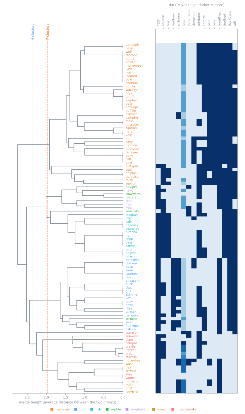
leaves_list returns the leaf order of the dendrogram, and the same trick clusters the columns: features that tend to be answered the same way (eggs, aquatic, fins; hair, milk, breathes, toothed) are placed side by side. The result is the table itself, with nothing added and nothing removed, but read in an order in which its structure is visible: solid blocks for hair and milk down the mammals, feathers down the birds, fins down the fish, and the empty backbone column down the invertebrates. The colors of the names show the audit of step 8 at a glance.
Your turn
- A distance for yes/no data. The 15 yes/no columns can be compared with the Jaccard distance (the fraction of disagreements among the questions where at least one of the two animals says yes). Build
linkage(Xs[:, yes_no].astype(bool), 'average', metric='jaccard'), cut it at 7 and compare its ARI againstkindwith step 8. Why can't you use'ward'with this metric? - Single linkage on the zoo. Cut
trees['single']at \(k = 4\) and \(k = 7\) and print the cluster sizes. Where does chaining show up? Relate what you see to its cophenetic correlation in step 3, which was not the lowest. - StandardScaler instead. Redo steps 3–8 with
StandardScaler. Does the ARI at \(k = 7\) go up or down? Which features gained weight, and does that make zoological sense? - Remove the duplicates. Drop the 42 duplicate rows (
X.duplicated()), rebuild the average tree and compare the gap/silhouette table with step 5. Which numbers change, and why do the duplicates matter for the silhouette but not for the shape of the tree?
Class materials
Lab notebook and handouts (in Portuguese)
- Lab notebook of this lesson: lab-hierarchical-clustering.ipynb — download it and open it in Jupyter or Colab (File → Upload notebook).
- Handout — Agrupamento e k-means: its closing panorama places hierarchical clustering among the other families of methods and compares Ward with k-means, GMM, spectral clustering and HDBSCAN on five shapes: handout
- Lab — Agrupar 178 vinhos: its step 7 audits Ward against k-means and GMM on the wine data, and its second challenge clusters a co-association matrix with average linkage: open the challenge
References
- Ward, J. H., Jr. "Hierarchical Grouping to Optimize an Objective Function." Journal of the American Statistical Association 58, no. 301 (1963): 236–244 — the merge that raises the sum of squares least. DOI
- Sokal, R. R.; Rohlf, F. J. "The Comparison of Dendrograms by Objective Methods." Taxon 11, no. 2 (1962): 33–40 — the cophenetic correlation. DOI
- Lance, G. N.; Williams, W. T. "A General Theory of Classificatory Sorting Strategies: 1. Hierarchical Systems." The Computer Journal 9, no. 4 (1967): 373–380 — one update formula for all the linkages. DOI
- Gower, J. C.; Ross, G. J. S. "Minimum Spanning Trees and Single Linkage Cluster Analysis." Journal of the Royal Statistical Society, Series C (Applied Statistics) 18, no. 1 (1969): 54–64 — single linkage is the minimum spanning tree. DOI
- Müllner, D. "Modern Hierarchical, Agglomerative Clustering Algorithms." (2011) — the algorithms behind SciPy's
linkageand their complexity. arXiv:1109.2378 - Forsyth, R. "Zoo." UCI Machine Learning Repository (1990) — the lab's dataset (OpenML 42667). DOI