The path of this part
- Match the linkage to the shapechaining against compact groups; a local rule for the cut
- Choose the distanceone update formula; correlation and cosine
- Face the costquadratic memory and time; sample, then assign
- Choose the toolagainst k-means and density-based clustering; applications
Linkage behaviors, measured
Four datasets with known groups, 300 points each, every method told the true number of clusters. Score: the ARI (Adjusted Rand Index): 1 for the true groups, about 0 for chance.
| single | complete | average | Ward | |
|---|---|---|---|---|
| blobs | 0.57 | 0.98 | 0.98 | 0.98 |
| blobs + bridge | 0.00 | 0.91 | 0.99 | 0.96 |
| moons | 1.00 | 0.20 | 0.43 | 0.30 |
| parallel strips | 1.00 | 0.12 | 0.19 | 0.22 |
Two camps
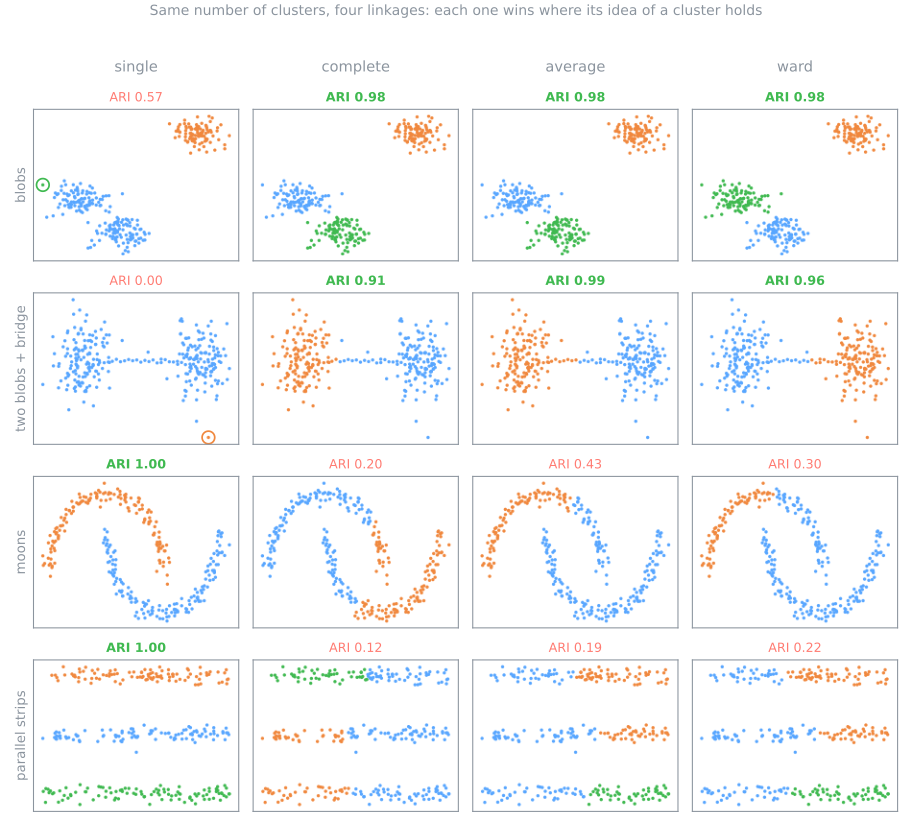
Single asks "is there some short hop?": it follows chains (1.00 on moons and strips), and a bridge of 20 points merges two blobs (0.00). That is chaining.
Complete, average, Ward compare the groups as a whole: a bridge cannot pull blobs together, but they cut moons and strips across, as k-means does.
A local rule for the cut: the inconsistency coefficient
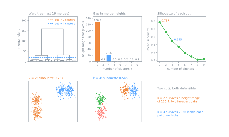
\(h\) = height of a merge; \(\bar h\), \(s\) = mean and standard deviation of \(h\) and the heights of the merges just below it (depth 2: at most three heights). Ward tree of the 400 points.
| merge | \(\bar h\) | \(s\) | coef. |
|---|---|---|---|
| 4th from top | 7.05 | 3.05 | 0.86 |
| 3rd | 16.14 | 12.22 | 1.15 |
| 2nd | 16.90 | 13.36 | 1.15 |
| top | 73.93 | 73.87 | 1.15 |
One update formula for every linkage
After \(I\) and \(J\) merge, the distance from any other cluster \(K\) to \(I \cup J\) (Lance & Williams, 1967), with coefficients \(\alpha_I, \alpha_J, \beta, \gamma\) chosen by the linkage:
\[ d(K, I \cup J) = \alpha_I\, d(K, I) + \alpha_J\, d(K, J) + \beta\, d(I, J) + \gamma\, \lvert d(K, I) - d(K, J) \rvert \]| linkage | coefficients | \(d(C, \{A, B\})\) |
|---|---|---|
| single | \(\alpha = \tfrac12,\ \beta = 0,\ \gamma = -\tfrac12\) | \(3.5 + 2 - 1.5 = 4\) |
| complete | \(\alpha = \tfrac12,\ \beta = 0,\ \gamma = +\tfrac12\) | \(3.5 + 2 + 1.5 = 7\) |
| average | \(\alpha_I = \tfrac{|I|}{|I| + |J|},\ \beta = \gamma = 0\) | \(3.5 + 2 = 5.5\) |
Beyond Euclidean distance
profiles: correlation distance
Four customers: two grow steadily, two spend in one peak month; one of each spends five times more.
Euclidean groups by how much they spend; \(1 - r\) groups by the shape.
documents: cosine distance
A text, the same text ten times longer, a text on another topic. From the first, Euclidean: 20.12 to the long copy, 3.87 to the other topic. Cosine: 0.0 and 1.0.
Cost: why it does not scale
| rows | pairwise distances |
|---|---|
| 1,000 | 0.004 GB |
| 10,000 | 0.400 GB |
| 100,000 | 40 GB |
| 1,000,000 | about 4,000 GB |
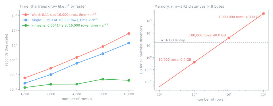
The best algorithms are \(O(n^2)\), still quadratic. On the machine that drew the figure, 16,000 rows took 6.11 s with Ward; k-means, 0.004 s. A method for hundreds to tens of thousands of rows.
What to do with more rows
- Sample, then assign. Tree on a 2% sample (2,000 of 100,000 rows), cut into 5, every other row to the nearest centroid: ARI 0.993. What you lose is the fine structure: a group of 30 points would have about 0.6 representatives.
- Connectivity constraints: merge only neighbors in a sparse graph.
- HDBSCAN (hierarchical DBSCAN, density-based spatial clustering of applications with noise) is itself hierarchical: a single-linkage tree on a density-adjusted distance, without the full matrix, and it marks noise.
Hierarchical vs k-means vs DBSCAN
| hierarchical | k-means | DBSCAN / HDBSCAN | |
|---|---|---|---|
| a cluster is | a branch of the merge tree | the points nearest one centroid | a dense region |
| decided after fitting | \(k\) or the cut height | — | — |
| output | a nested family of partitions | one partition | one partition + noise |
| any distance? | yes, except Ward | Euclidean only | yes |
| new points | no predict | predict | no predict |
| same result every run | yes | depends on the start | yes |
Applications
Taxonomies: whenever the product is a tree, not a partition.
Segmentation at several granularities: 12 fine segments that are subdivisions of 3 coarse ones.
Gene-expression heat maps: cluster rows and columns with correlation distance and redraw in leaf order.
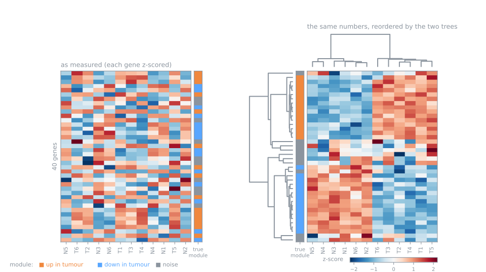
Same numbers, reordered by the tree: blocks of genes up and down in tumours appear, and the column tree splits tumour from normal samples at its top merge.
Summary
- Single follows chains and is fooled by bridges; complete, average and Ward find compact groups and cut thin shapes across.
- A local rule for the cut (the inconsistency coefficient) misses what the gaps, read from the top, see.
- One update formula: any dissimilarity works, except for Ward. Correlation distance for profiles, cosine for documents.
- Quadratic memory and time: hundreds to tens of thousands of rows. Beyond that: sample and assign, connectivity constraints, HDBSCAN.
- Choose a tree when the product is a hierarchy, the groups are unequal, or several levels of detail are needed.
The tree against k-means and the answer key, steps 7 to 9
- Same notebook, same session, from step 7.
- Step 7: k-means with \(k = 4\) and \(k = 7\); do its partitions nest like the tree's cuts?
- Step 8: open the zoologists' classes and audit every decision of the fundamental lab.
- Step 9: the heat map, rows and columns reordered by the tree.
- Simulations: k-means with another seed (step 7) and the linkage, audited (step 8).
Pace: step 7 and its simulation in 10 min; step 8 and its simulation in 10 min; step 9 in 5 min.