Machine Learning · Insper

Hierarchical Clustering

Fundamental approach

How merging the closest pair, again and again, builds a tree, and how the tree becomes groups

From one partition to a tree

k-means

needs \(k\) before it starts; returns one flat partition

hierarchical

builds all the groupings at once, nested, as a tree: the dendrogram. \(k\) is chosen afterwards, by cutting it.

The oldest way of organizing living things: kingdoms, classes, orders, families, species. Still what biologists, librarians and marketing teams want when one level of detail is not enough.

The path of this part

Build the treemerge the closest pair; four linkages by hand
Read the treeheights, not leaf order; the matrix Z
Cut ita horizontal line; the gaps and the silhouette
Check ithow faithfully the heights keep the distances

Each stage answers one question: how does merging, pair by pair, build a tree? → what does the tree say? → how does the tree become groups? → how faithful is the tree to the distances?

Stage 1 · how does merging, pair by pair, build a tree?

The idea: merge the two closest groups, repeat

start with \(n\) clusters, one per point;
find the two clusters closest to each other;
merge them, and record the distance: the merge height;
repeat until one cluster is left.

After \(n - 1\) merges, the history of the merges is the tree. Nothing random, nothing iterated to convergence: the same data always gives the same tree (up to ties).

Step 2 hides the only real decision: the distance between two clusters.

The linkage: distance between clusters

linkage	distance between \(P\) and \(Q\)	tends to produce
single	the closest pair	chains; one bridge merges two groups
complete	the farthest pair	compact groups of similar diameter
average	the mean of all cross distances	a compromise
Ward	how much the merge raises the within-cluster sum of squares	round groups of similar size, like k-means

\[ \Delta(P, Q) = \frac{|P|\,|Q|}{|P| + |Q|}\, \lVert \mu_P - \mu_Q \rVert^2 \]

The within-cluster sum of squares is the k-means inertia: Ward grows it as slowly as it can, one greedy merge at a time.

Simulator: merge, watch the tree grow, cut it

Predict. On the chain (two blobs and a bridge), which linkage will glue the two blobs together long before the last merge?

Five points, four linkages, step by step

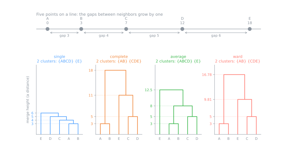
A = 0, B = 3, C = 7, D = 12, E = 18 on a line: the gaps grow by one. Predict. After A + B, which merge comes next for each linkage? Then step through and switch the linkage.

One matrix, different trees

The five points and the four dendrograms; cut into two clusters, single and average give {ABCD}{E}, complete and Ward give {AB}{CDE}

Asked for two clusters: single and average isolate E; complete and Ward cut between B and C. Neither is wrong: they answer different definitions of "a cluster".

Stage 2 · what does the tree say?

Reading a dendrogram

The y-axis is a distance. Two points are as similar as the height of the lowest bar that joins them: the cophenetic distance. Complete tree: A and B at 3, A and E at 18.
Long vertical lines are the interesting part: a group that stays far from everything. {C, D, E} forms at 11 and waits until 18.
The left-to-right order carries almost no information: each bar can flip, so 5 leaves have \(2^4 = 16\) equivalent drawings.

In the complete tree, E is drawn right next to B, although they end up 18 apart. Read similarity from the height where they meet, never from neighboring leaves.

The linkage matrix `Z`


Z = linkage(X, 'complete')
# [[ 0.  1.  3.  2.]
#  [ 2.  3.  5.  2.]
#  [ 4.  6. 11.  3.]
#  [ 5.  7. 18.  5.]]

column	meaning
0, 1	the two clusters merged; ids 0 to \(n-1\) are points, row \(i\) creates cluster \(n + i\)
2	the merge height: 3, 5, 11, 18
3	how many points the new cluster has: 2, 2, 3, 5

One row per merge, \(n - 1\) rows, in the order the merges happened.

Stage 3 · how does the tree become groups?

Cutting the tree

A horizontal line at height \(t\): each piece hanging below it is one cluster.

Predict. Complete tree (heights 3, 5, 11, 18). Which clusters does a cut at 8 give?

cut at	clusters
4	{A, B}, {C}, {D}, {E}
8	{A, B}, {C, D}, {E}
12	{A, B}, {C, D, E}
20	everything

Any cut between 11 and 18 gives the same two clusters: a range 7 units wide. That width is what makes the two-cluster answer stable here.

In scikit-learn, and one property


AgglomerativeClustering(n_clusters=2, linkage='ward').fit(X)
AgglomerativeClustering(n_clusters=None, distance_threshold=8, linkage='complete').fit(X)

The same merge heights as the hand tables (Ward on the \(\sqrt{2\Delta}\) scale).
No predict: a new point has no place in the tree until you rebuild it or assign it with another rule.

Cuts of the same tree are nested: the 3-cluster cut is the 2-cluster cut with one cluster split. Two k-means runs with \(k = 3\) and \(k = 4\) have no such obligation.

Choosing where to cut

400 points in four blobs that come in two pairs: two scales of structure. Ward tree.

\(k\)	range of cut heights	gap	silhouette
2	32.3 to 159.2	126.9	0.787
3	30.3 to 32.3	2.1	0.664
4	9.7 to 30.3	20.6	0.545
5	9.2 to 9.7	0.5	0.473

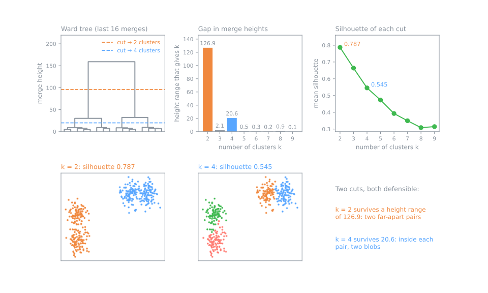
Ward tree of 400 points with cuts at 2 and 4 clusters; gap 126.9 for k=2 and 20.6 for k=4; silhouette falling from 0.787 to 0.545

The wider the range of heights a \(k\) survives, the more the data insist on it. The silhouette prefers the coarsest split and does not see the second scale.

So which cut is right?

Both: the cuts are nested. Report two segments at the coarse level and four at the fine level; they agree.
When one number is required, choose with the question in mind (how many groups can someone act on?) and use the gaps and the silhouette to rule out cuts the data do not support: \(k = 3\), gap 2.1.

Stage 4 · how faithful is the tree to the distances?

Cophenetic correlation, pair by pair

\(d\) = original distance of a pair; \(c\) = its cophenetic distance, the height where the two points first join. The cophenetic correlation is the correlation between \(d\) and \(c\) over the 10 pairs. Predict. Does the chain-shaped single tree keep the distances better or worse than the complete tree?

Faithful tree ≠ good clusters

The four blobs of the previous slides, four linkages. ARI (adjusted Rand index): 1 = the true groups, about 0 = chance.

	cophenetic correlation	ARI at \(k = 4\)
single	0.944	0.496
complete	0.947	0.954
average	0.953	0.856
Ward	0.952	0.892

The cophenetic correlation measures how faithfully the tree represents the distances, not how good the clusters are. Use it when the tree itself is the product: a taxonomy, the order of a heat map.

Summary

Merge the two closest clusters, repeat: the history of the merges is the tree.
The linkage defines "closest" and decides what the tree finds: one matrix, three trees.
Read heights, not the left-to-right order: two points are as similar as the bar where they meet.
A cut is a partition, and the cuts of one tree are nested; the widest range of heights points to \(k\).
Cophenetic correlation = how faithful the tree is to the distances, not how good the clusters are.

symptom	what to do
every \(k\) survives only a narrow range of heights	report the tree; do not force one \(k\)
two cuts, both with wide gaps	keep both levels: they are nested

Fundamental lab · about 30 min, in pairs

A tree of 101 animals, steps 1 to 6

The UCI (University of California, Irvine) Zoo table: 15 yes/no questions and the number of legs. The zoologists' class stays sealed until step 8, in the advanced part.
Scale the columns, build four trees and keep the most faithful, draw it, choose the cut and name the clusters.
Download the lab notebook and open it in Jupyter or Colab.
At every step, answer the Predict before running.
Simulations: the tree without scaling (step 2) and a new animal, without predict (step 6).

Pace: steps 1 and 2 and the first simulation in 10 min; steps 3 to 5 in 10 min; step 6 and the second simulation in 10 min.