From one partition to a tree
k-means
needs \(k\) before it starts; returns one flat partition
hierarchical
builds all the groupings at once, nested, as a tree: the dendrogram. \(k\) is chosen afterwards, by cutting it.
The path of this lesson
- Build the treemerge the closest pair; four linkages by hand
- Read and cutthe dendrogram, the matrix Z, the cut
- Choose and checklinkage behaviors, where to cut, cophenetic correlation
- In practiceother distances, cost, against k-means and density-based clustering
The idea: merge the two closest groups, repeat
- start with \(n\) clusters, one per point;
- find the two clusters closest to each other;
- merge them, and record the distance: the merge height;
- repeat until one cluster is left.
After \(n - 1\) merges, the history of the merges is the tree. Nothing random, nothing iterated to convergence: the same data always gives the same tree (up to ties).
The linkage: distance between clusters
| linkage | distance between \(P\) and \(Q\) | tends to produce |
|---|---|---|
| single | the closest pair | chains; one bridge merges two groups |
| complete | the farthest pair | compact groups of similar diameter |
| average | the mean of all cross distances | a compromise |
| Ward | how much the merge raises the within-cluster sum of squares | round groups of similar size, like k-means |
The within-cluster sum of squares is the k-means inertia: Ward grows it as slowly as it can, one greedy merge at a time.
Simulator: merge, watch the tree grow, cut it
Predict. On the chain (two blobs and a bridge), which linkage will glue the two blobs together long before the last merge?
Five points on a line
| point | A | B | C | D | E |
|---|---|---|---|---|---|
| position | 0 | 3 | 7 | 12 | 18 |
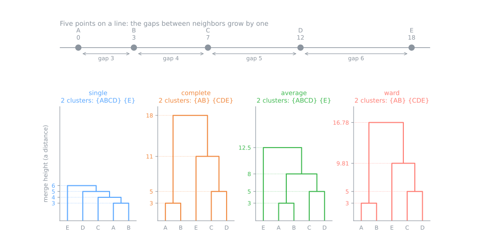
The gaps grow by one: 3, 4, 5, 6. Exactly where the linkages disagree.
| A | B | C | D | E | |
|---|---|---|---|---|---|
| A | 0 | 3 | 7 | 12 | 18 |
| B | 3 | 0 | 4 | 9 | 15 |
| C | 7 | 4 | 0 | 5 | 11 |
| D | 12 | 9 | 5 | 0 | 6 |
| E | 18 | 15 | 11 | 6 | 0 |
Merge 2 already splits the linkages
The new row: the distance from \(\{A, B\}\) to everything else.
| from {A, B} to | single = min | complete = max | average = mean |
|---|---|---|---|
| C | min(7, 4) = 4 | 7 | 5.5 |
| D | 9 | 12 | 10.5 |
| E | 15 | 18 | 16.5 |
The rest of the matrix does not change: C–D = 5, C–E = 11, D–E = 6.
Single: the smallest entry is 4, so C joins {A, B}. Complete and average: their row is larger, the smallest entry is C–D = 5, so C pairs with D.
Four trees, to the end
| linkage | merges | heights |
|---|---|---|
| single | AB → ABC → ABCD → ABCDE | 3, 4, 5, 6 |
| complete | AB → CD → CDE → all | 3, 5, 11, 18 |
| average | AB → CD → ABCD → all | 3, 5, 8, 12.5 |
| Ward | AB → CD → CDE → all | 3, 5, 9.81, 16.78 |
- Merge 3: average joins the two pairs (8 against 8.5); complete sees the 12 between A and D and brings E into {C, D} (11).
- Ward's costs \(\Delta\): 4.5 + 12.5 + 48.17 + 140.83 = 206, the sum of squares of the five points around their mean 8. The height reported is \(\sqrt{2\Delta}\): \(\sqrt{2 \cdot 4.5} = 3\).
One matrix, different trees
Reading a dendrogram
- The y-axis is a distance. Two points are as similar as the height of the lowest bar that joins them: the cophenetic distance. Complete tree: A and B at 3, A and E at 18.
- Long vertical lines are the interesting part: a group that stays far from everything. {C, D, E} forms at 11 and waits until 18.
- The left-to-right order carries almost no information: each bar can flip, so 5 leaves have \(2^4 = 16\) equivalent drawings.
The linkage matrix Z
Z = linkage(X, 'complete')
# [[ 0.  1.  3.  2.]
#  [ 2.  3.  5.  2.]
#  [ 4.  6. 11.  3.]
#  [ 5.  7. 18.  5.]]
| column | meaning |
|---|---|
| 0, 1 | the two clusters merged; ids 0 to \(n-1\) are points, row \(i\) creates cluster \(n + i\) |
| 2 | the merge height: 3, 5, 11, 18 |
| 3 | how many points the new cluster has: 2, 2, 3, 5 |
One row per merge, \(n - 1\) rows, in the order the merges happened.
Cutting the tree
A horizontal line at height \(t\): each piece hanging below it is one cluster.
| cut at | clusters |
|---|---|
| 4 | {A, B}, {C}, {D}, {E} |
| 8 | {A, B}, {C, D}, {E} |
| 12 | {A, B}, {C, D, E} |
| 20 | everything |
Any cut between 11 and 18 gives the same two clusters: a range 7 units wide. That width is what makes the two-cluster answer stable here.
In scikit-learn, and one property
AgglomerativeClustering(n_clusters=2, linkage='ward').fit(X)
AgglomerativeClustering(n_clusters=None, distance_threshold=8, linkage='complete').fit(X)
- The same merge heights as the hand tables (Ward on the \(\sqrt{2\Delta}\) scale).
- No
predict: a new point has no place in the tree until you rebuild it or assign it with another rule.
Linkage behaviors, measured
Four datasets with known groups, 300 points each, every method told the true number of clusters. Score: the ARI (Adjusted Rand Index): 1 for the true groups, about 0 for chance.
| single | complete | average | Ward | |
|---|---|---|---|---|
| blobs | 0.57 | 0.98 | 0.98 | 0.98 |
| blobs + bridge | 0.00 | 0.91 | 0.99 | 0.96 |
| moons | 1.00 | 0.20 | 0.43 | 0.30 |
| parallel strips | 1.00 | 0.12 | 0.19 | 0.22 |
Two camps
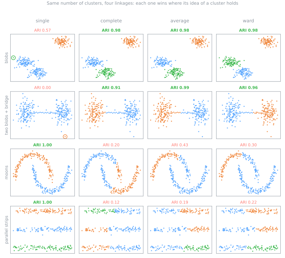
Single asks "is there some short hop?": it follows chains (1.00 on moons and strips), and a bridge of 20 points merges two blobs (0.00). That is chaining.
Complete, average, Ward compare the groups as a whole: a bridge cannot pull blobs together, but they cut moons and strips across, as k-means does.
Choosing where to cut
400 points in four blobs that come in two pairs: two scales of structure. Ward tree.
| \(k\) | range of cut heights | gap | silhouette |
|---|---|---|---|
| 2 | 32.3 to 159.2 | 126.9 | 0.787 |
| 3 | 30.3 to 32.3 | 2.1 | 0.664 |
| 4 | 9.7 to 30.3 | 20.6 | 0.545 |
| 5 | 9.2 to 9.7 | 0.5 | 0.473 |
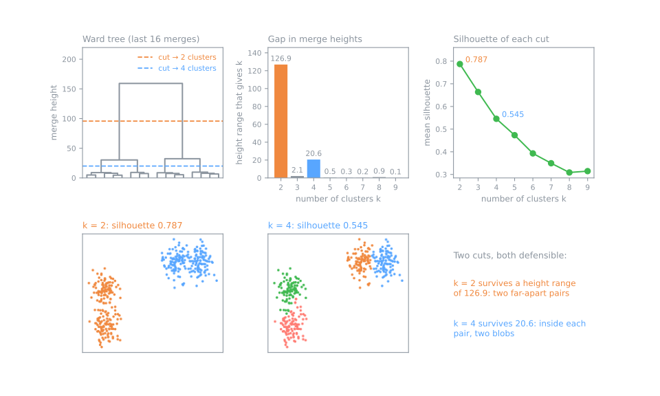
The wider the range of heights a \(k\) survives, the more the data insist on it. The silhouette prefers the coarsest split and does not see the second scale.
So which cut is right?
- Both: the cuts are nested. Report two segments at the coarse level and four at the fine level; they agree.
- When one number is required, choose with the question in mind (how many groups can someone act on?) and use the gaps and the silhouette to rule out cuts the data do not support: \(k = 3\), gap 2.1.
- The inconsistency coefficient is local: with depth 2 it cannot exceed \(2/\sqrt3 = 1.15\), and the top three merges all reach it. One more hint, at most.
Cophenetic correlation: how faithful is the tree?
The correlation between the original distances and the cophenetic ones. By hand, single-linkage tree of the five points:
| AB | AC | AD | AE | BC | BD | BE | CD | CE | DE | |
|---|---|---|---|---|---|---|---|---|---|---|
| original \(d\) | 3 | 7 | 12 | 18 | 4 | 9 | 15 | 5 | 11 | 6 |
| cophenetic \(c\) | 3 | 4 | 5 | 6 | 4 | 5 | 6 | 5 | 6 | 6 |
\(33 / \sqrt{220 \times 10} = \mathbf{0.704}\). The other trees: complete 0.565, average 0.691, Ward 0.561.
Faithful tree ≠ good clusters
The four blobs, four linkages:
| cophenetic correlation | ARI at \(k = 4\) | |
|---|---|---|
| single | 0.944 | 0.496 |
| complete | 0.947 | 0.954 |
| average | 0.953 | 0.856 |
| Ward | 0.952 | 0.892 |
Beyond Euclidean distance
profiles: correlation distance
Four customers: two grow steadily, two spend in one peak month; one of each spends five times more.
Euclidean groups by how much they spend; \(1 - r\) groups by the shape.
documents: cosine distance
A text, the same text ten times longer, a text on another topic. From the first, Euclidean: 20.12 to the long copy, 3.87 to the other topic. Cosine: 0.0 and 1.0.
Cost: why it does not scale
| rows | pairwise distances |
|---|---|
| 1,000 | 0.004 GB |
| 10,000 | 0.400 GB |
| 100,000 | 40 GB |
| 1,000,000 | about 4,000 GB |
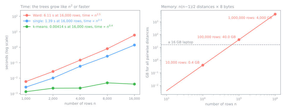
The best algorithms are \(O(n^2)\), still quadratic. On the machine that drew the figure, 16,000 rows took 6.11 s with Ward; k-means, 0.004 s. A method for hundreds to tens of thousands of rows.
What to do with more rows
- Sample, then assign. Tree on a 2% sample (2,000 of 100,000 rows), cut into 5, every other row to the nearest centroid: ARI 0.993. What you lose is the fine structure: a group of 30 points would have about 0.6 representatives.
- Connectivity constraints: merge only neighbors in a sparse graph.
- HDBSCAN (hierarchical DBSCAN, density-based spatial clustering of applications with noise) is itself hierarchical: a single-linkage tree on a density-adjusted distance, without the full matrix, and it marks noise.
Hierarchical vs k-means vs DBSCAN
| hierarchical | k-means | DBSCAN / HDBSCAN | |
|---|---|---|---|
| a cluster is | a branch of the merge tree | the points nearest one centroid | a dense region |
| decided after fitting | \(k\) or the cut height | — | — |
| output | a nested family of partitions | one partition | one partition + noise |
| any distance? | yes, except Ward | Euclidean only | yes |
| new points | no predict | predict | no predict |
| same result every run | yes | depends on the start | yes |
Applications
Taxonomies: whenever the product is a tree, not a partition.
Segmentation at several granularities: 12 fine segments that are subdivisions of 3 coarse ones.
Gene-expression heat maps: cluster rows and columns with correlation distance and redraw in leaf order.
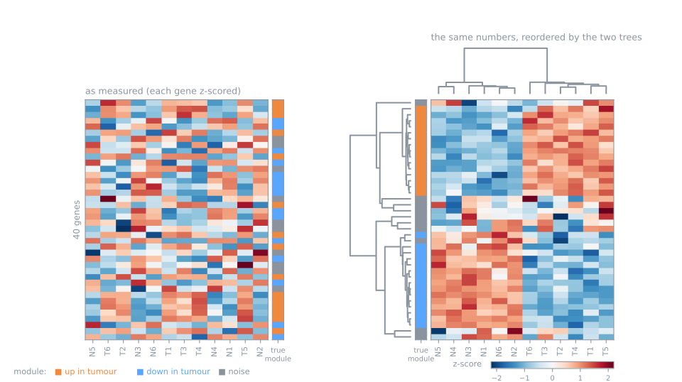
Same numbers, reordered by the tree: blocks of genes up and down in tumours appear, and the column tree splits tumour from normal samples at its top merge.
Summary
- Merge the two closest clusters, repeat: the history of merges is the tree.
- The linkage defines "closest" and decides what the tree finds.
- Read heights, not the left-to-right order; cuts of one tree are nested.
- Choose the cut by the gaps in merge heights, with the question in mind.
- Cophenetic correlation = fidelity of the tree, not quality of the clusters.
- Quadratic cost: hundreds to tens of thousands of rows.
A tree of 101 animals
- The UCI (University of California, Irvine) Zoo table: 15 yes/no questions and the number of legs. The zoologist's class is sealed until step 8.
- Can a tree of 16 plain features rediscover the taxonomy? What does it show that k-means does not?
- Download the lab notebook and open it in Jupyter or Colab.
1. load and look
2. the columns on the same scale
3. four linkages, how faithful each tree is
4. draw the tree
5. choose the cut: gaps and silhouette
6. profile the clusters
7. the same data with k-means
8. open the answer key
9. the heat map, reordered by the tree