k-Nearest Neighbors
The logistic regression of the previous lesson reads the whole training set, sums it up in a handful of numbers (one weight per feature plus an intercept), draws a straight line and throws the rows away. k-NN (Fix & Hodges, 1951; Cover & Hart, 1967) does the opposite: it keeps every training row, and to classify a new point it looks up the \(k\) most similar rows and lets them vote. There are no weights to fit and no training loop. The "model" is the training data, which is why the decision boundary can take any shape the data suggests.
Every claim below is measured: each figure is produced by a short Python script next to this page, and the code blocks print the numbers quoted in the text.
How this lesson is organized
The lesson has two approaches. Each one has slides, text and a lab to run in class on Colab; the quiz at the end covers the fundamental one. Start with the fundamental one: the advanced one builds on it.
| Fundamental approach | Advanced approach | |
|---|---|---|
| question | How does k-NN decide, and what does it need to decide well? | Where does k-NN break, what does it cost, and when should you use another model? |
| content | the neighbors' vote, what fit stores, scaling, choosing \(k\) | other distances, ties and weights, predict_proba, the curse of dimensionality, cost, k-NN vs logistic regression, regression |
| in-class lab | wines, steps 1 to 5 | handwritten digits, steps 6 to 8 |
| by the end, you can | predict by hand with \(k\) = 1, 3 and 5; build the right pipeline; choose \(k\) on validation and test once | choose the distance; read ties, weights and probabilities; diagnose high dimension; decide between k-NN and logistic regression |
Both labs use the same notebook on Colab (in Portuguese): the fundamental part runs steps 1 to 5, the advanced part steps 6 to 8. Everything runs in the browser; there is nothing to download.
Fundamental approach
One question guides this part: how does k-NN decide, and what does it need to decide well? Four ideas answer it: the neighbors vote; fit only stores the data; distances require features on the same scale; \(k\) is chosen on a validation split.
The four ideas come in three stages, drawn below: 1. the neighbors vote (and fit only stores the rows); 2. scale first, so that every feature counts in the distance; 3. choose \(k\) on validation and test once. Each stage links to its section, and in the slides a strip at the bottom shows which stage you are in.
- Neighbors votedistance to every row; the k nearest vote;
fitonly stores - Scale firstunits decide the distance; the scaler goes inside a pipeline
- Choose k, test oncebias and variance; validation chooses, the test confirms
Slides: fundamental approach
Click the slides and use the ← → arrows to navigate; F goes full screen and Esc shows every slide. Open the slides in a new tab
1. The idea, worked by hand
Stage 1. A streaming service is about to recommend a new series that mixes action and documentary. It knows, for ten subscribers who have already watched it, how many hours of action films and of documentaries they watch per week, and whether they liked the series. A new subscriber watches 4 hours of action and 4 hours of documentaries. Will they like it?
Measure how far each known subscriber is from the new one with the ordinary (Euclidean) distance, \(d = \sqrt{(\text{action} - 4)^2 + (\text{docs} - 4)^2}\), and sort:
| rank | name | action | docs | liked? | \(d^2\) | \(d\) |
|---|---|---|---|---|---|---|
| 1 | Ana | 5 | 4 | yes | 1 + 0 = 1 | 1.000 |
| 2 | Bruno | 2 | 5 | no | 4 + 1 = 5 | 2.236 |
| 3 | Carla | 6 | 6 | no | 4 + 4 = 8 | 2.828 |
| 4 | Davi | 4 | 7 | yes | 0 + 9 = 9 | 3.000 |
| 5 | Elisa | 7 | 3 | yes | 9 + 1 = 10 | 3.162 |
| 6 | Felipe | 1 | 2 | no | 9 + 4 = 13 | 3.606 |
| 7 | Gabi | 8 | 6 | yes | 16 + 4 = 20 | 4.472 |
| 8 | Hugo | 1 | 8 | no | 9 + 16 = 25 | 5.000 |
| 9 | Iara | 9 | 2 | yes | 25 + 4 = 29 | 5.385 |
| 10 | João | 1 | 9 | no | 9 + 25 = 34 | 5.831 |
Now let the \(k\) nearest vote:
- \(k = 1\): only Ana votes. She liked it, so the prediction is liked;
- \(k = 3\): Ana (yes), Bruno (no), Carla (no). Two against one: not liked;
- \(k = 5\): add Davi (yes) and Elisa (yes). Three against two: liked again.
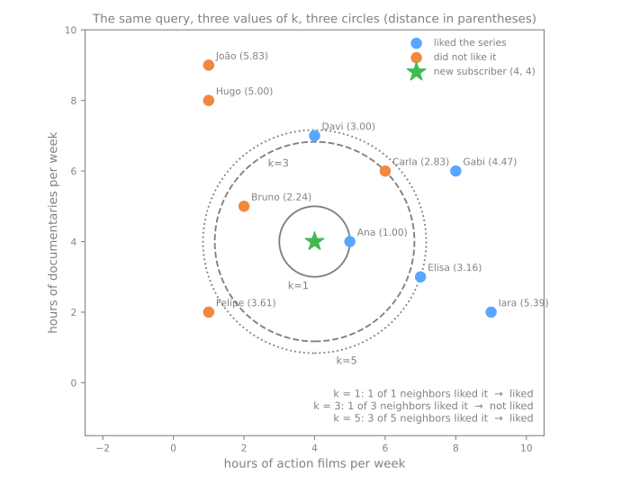
Same data, same query, three different answers. \(k\) is not a detail: it is the main decision k-NN leaves to you. scikit-learn confirms the hand computation:
import numpy as np
import pandas as pd
from sklearn.neighbors import KNeighborsClassifier

users = pd.DataFrame({
    'name':   ['Ana', 'Bruno', 'Carla', 'Davi', 'Elisa', 'Felipe', 'Gabi', 'Hugo', 'Iara', 'João'],
    'action': [5, 2, 6, 4, 7, 1, 8, 1, 9, 1],      # hours of action films per week
    'docs':   [4, 5, 6, 7, 3, 2, 6, 8, 2, 9],      # hours of documentaries per week
    'liked':  [1, 0, 0, 1, 1, 0, 1, 0, 1, 0]})     # 1 = liked the new series
X, y = users[['action', 'docs']], users['liked']
new = pd.DataFrame({'action': [4], 'docs': [4]})

knn = KNeighborsClassifier(n_neighbors=5).fit(X, y)
dist, idx = knn.kneighbors(new)                    # the 5 nearest, in order
print(users['name'].iloc[idx[0]].tolist(), dist[0].round(3))

for k in [1, 3, 5]:
    knn = KNeighborsClassifier(n_neighbors=k).fit(X, y)
    print(f"k={k}: predict {knn.predict(new)[0]}   P(liked) = {knn.predict_proba(new)[0, 1]:.3f}")
['Ana', 'Bruno', 'Carla', 'Davi', 'Elisa'] [1.    2.236 2.828 3.    3.162]
k=1: predict 1   P(liked) = 1.000
k=3: predict 0   P(liked) = 0.333
k=5: predict 1   P(liked) = 0.600
kneighbors returns the same five names, in the same order, at the same distances as the table. predict_proba is nothing more than the share of the \(k\) neighbors who liked the series: 1/1, 1/3 and 3/5.
Key idea
k-NN does not learn a formula: it looks up the cases most similar to the new point and repeats the answer of most of them. Changing \(k\) changes who votes and, near the boundary, changes the answer.
2. The algorithm in three steps
To classify a query point \(x\):
- compute the distance from \(x\) to every training point;
- keep the \(k\) closest, the neighborhood \(N_k(x)\);
- predict the most frequent class among them. The "probability" of class \(c\) is the fraction of neighbors in that class:
In practice k-NN always goes in a pipeline with a scaler, for reasons measured further down:
from sklearn.neighbors import KNeighborsClassifier
from sklearn.pipeline import make_pipeline
from sklearn.preprocessing import StandardScaler

knn = make_pipeline(StandardScaler(),                 # distances need scaling!
                    KNeighborsClassifier(n_neighbors=5))
knn.fit(X_train, y_train)
What fit stores: parametric vs instance-based
Logistic regression is a parametric model: whatever the size of the training set, what it learns fits in \(d + 1\) numbers. k-NN is instance-based (or non-parametric): what it "learns" is the training set itself, so the model grows with the data.
| logistic regression | k-NN | |
|---|---|---|
what fit produces | \(d + 1\) numbers (\(w\), \(b\)) | a copy of the \(n \times d\) training table |
| decision boundary | a straight line (hyperplane) | any shape; follows the data locally |
cost of fit | iterative optimization | almost none: store the rows |
| cost of one prediction | \(d\) multiplications | \(n\) distances of \(d\) coordinates each |
| knobs | none in its plain form: you choose the features | k, the distance, the weighting |
| can say why | one coefficient per feature | "these \(k\) rows are the most similar" |
The table sums up k-NN's nickname: it is a lazy learner. fit optimizes nothing; at most it organizes the rows to speed up the search. The real work, computing the distance from the query to the stored rows, is left for prediction time. The advanced approach counts those distances and shows what they cost.
3. Scaling is not optional
Stage 2. A distance adds up differences in the units of each feature. When the units differ, the feature with the largest numbers decides everything. Consider six customers of a travel agency (some bought a backpacking package, some did not) and a new customer (R$ 5,000 per month, 25 years old). Will they buy?
from sklearn.preprocessing import StandardScaler

clients = pd.DataFrame({
    'name':   ['Rita', 'Otávio', 'Sônia', 'Caio', 'Lívia', 'Mário'],
    'income': [5200, 5700, 9000, 3000, 7400, 2600],      # R$ per month
    'age':    [61, 26, 45, 33, 52, 22],
    'bought': [0, 1, 0, 1, 0, 1]})
F = ['income', 'age']
query = pd.DataFrame({'income': [5000], 'age': [25]})

scaler = StandardScaler().fit(clients[F])
Z, zq = scaler.transform(clients[F]), scaler.transform(query)
clients['d_raw'] = np.sqrt(((clients[F] - query.iloc[0]) ** 2).sum(axis=1)).round(1)
clients['d_scaled'] = np.sqrt(((Z - zq) ** 2).sum(axis=1)).round(2)
print(scaler.scale_.round(1))
print(clients.sort_values('d_raw').to_string(index=False))
[2260.1   14. ]
  name  income  age  bought  d_raw  d_scaled
  Rita    5200   61       0  203.2      2.57
Otávio    5700   26       1  700.0      0.32
  Caio    3000   33       1 2000.0      1.05
 Mário    2600   22       1 2400.0      1.08
 Lívia    7400   52       0 2400.2      2.20
 Sônia    9000   45       0 4000.0      2.27
Check Rita by hand: \(\sqrt{200^2 + 36^2} = \sqrt{40{,}000 + 1{,}296} = 203.2\). Her income is R$ 200 away and her age 36 years away, and the 36 years add only 3.2 to the distance, because one year weighs as much as one real. In raw units the nearest neighbor is a 61-year-old who did not buy, and 1-NN says "no".
StandardScaler divides each feature by its standard deviation (R$ 2,260.1 and 14.0 years here; the means cancel in a difference). Now Rita is \(\sqrt{(200/2260.1)^2 + (36/14.0)^2} = \sqrt{0.09^2 + 2.57^2} = 2.57\) away, and Otávio, 26 years old, \(\sqrt{(700/2260.1)^2 + (1/14.0)^2} = 0.32\). The nearest neighbor becomes a customer of almost the same age who bought, and 1-NN says "yes".
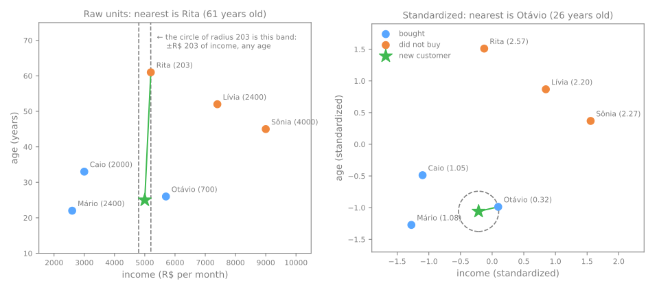
The left panel is the whole story: in raw units, a "circle" of radius 203 around the new customer is a band R$ 203 wide on each side that contains every age in the picture. On a real dataset the effect is just as large. The 13 features of the wine dataset have wildly different spreads:
from sklearn.datasets import load_wine
from sklearn.model_selection import train_test_split
from sklearn.pipeline import make_pipeline
from sklearn.preprocessing import MinMaxScaler

wine = load_wine(as_frame=True)
print(wine.data.std().sort_values(ascending=False).round(2).head(4))

X_tr, X_te, y_tr, y_te = train_test_split(wine.data, wine.target, test_size=0.3,
                                          stratify=wine.target, random_state=0)
for name, model in [('no scaling', KNeighborsClassifier(5)),
                    ('StandardScaler', make_pipeline(StandardScaler(), KNeighborsClassifier(5))),
                    ('MinMaxScaler', make_pipeline(MinMaxScaler(), KNeighborsClassifier(5)))]:
    print(f"{name:15s} {model.fit(X_tr, y_tr).score(X_te, y_te):.3f}")
proline              314.91
magnesium             14.28
alcalinity_of_ash      3.34
color_intensity        2.32
dtype: float64
no scaling      0.722
StandardScaler  0.963
MinMaxScaler    0.963
proline has a standard deviation of 315, more than twenty times that of any other feature, so the raw distance is essentially the proline difference: 5-NN is classifying wines by one column out of 13. It gets 72.2% of the 54 test wines right (39). Put the features on a common scale and the same 5-NN gets 96.3% (52). Standardization and min-max scaling do equally well here; what matters is that no feature dominates by accident of its unit.
Scale first, always, and inside a pipeline
k-NN without scaling is a bug, not a model (unless all features already share one unit, as the pixels in the advanced lab do). The scaler must learn its means and standard deviations from the training rows only, then be applied frozen to validation and test. make_pipeline(StandardScaler(), KNeighborsClassifier()) does exactly that (Pipelines).
4. Choosing \(k\): bias and variance
Stage 3. \(k\) is the complexity knob. A small \(k\) listens to very few points, so the boundary bends around each of them; a large \(k\) averages over a big region, so the boundary becomes smooth. It is the bias–variance trade-off with the direction reversed: small \(k\) = complex model. To see it, take a noisy two-moons dataset (1,000 points) and split it into 600 training, 200 validation and 200 test points:
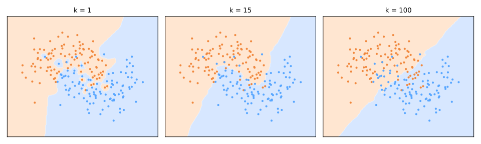
- \(k = 1\): every training point rules its own island. The boundary memorizes the noise; training accuracy is 100% and validation 85.0%: high variance, overfitting;
- \(k = 15\): a smooth boundary that follows the two moons, 89.5% on validation;
- \(k = 451\) (three quarters of the training set): each vote is swamped by the far side of the data, and the boundary is almost a straight line: high bias, underfitting. At \(k = n\) every query gets the same neighbors, and k-NN predicts the majority class everywhere.
To choose \(k\), score every candidate on the validation split. The test split stays untouched until the very end:
from sklearn.datasets import make_moons

X, y = make_moons(n_samples=1000, noise=0.35, random_state=0)
X_tmp, X_test, y_tmp, y_test = train_test_split(X, y, test_size=0.2, stratify=y, random_state=0)
X_train, X_val, y_train, y_val = train_test_split(X_tmp, y_tmp, test_size=0.25,
                                                  stratify=y_tmp, random_state=0)
print(len(X_train), len(X_val), len(X_test))

rows = []
for k in range(1, 452, 2):                                   # every odd k up to 451
    m = KNeighborsClassifier(n_neighbors=k).fit(X_train, y_train)
    rows.append((k, m.score(X_train, y_train), m.score(X_val, y_val)))
table = pd.DataFrame(rows, columns=['k', 'train', 'validation'])
print(table[table['k'].isin([1, 3, 5, 9, 15, 31, 51, 73, 101, 151, 301, 451])]
      .round(3).to_string(index=False))
600 200 200
  k  train  validation
  1  1.000       0.850
  3  0.913       0.865
  5  0.900       0.880
  9  0.890       0.890
 15  0.888       0.895
 31  0.887       0.890
 51  0.878       0.900
 73  0.878       0.910
101  0.880       0.890
151  0.865       0.875
301  0.827       0.835
451  0.772       0.765
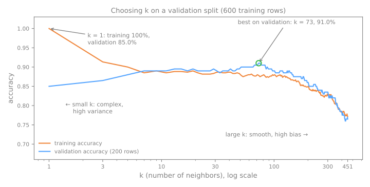
How to read it:
- Training accuracy at \(k = 1\) is 100% by construction. Each training point is its own nearest neighbor, at distance 0, so it always votes for its own label. That number says nothing about new data. The validation score, 85.0%, does.
- The plateau. From \(k = 7\) to \(k \approx 140\), validation accuracy stays between 88.5% and 91.0%. With 200 validation rows, one row is worth 0.5 points, so the whole plateau spans 5 rows: the data barely distinguishes these values of \(k\). The rule of thumb \(k \approx \sqrt{n} = \sqrt{600} \approx 24\) lands on the plateau too, but measure rather than trust it.
- Large \(k\). Beyond \(k \approx 150\), training and validation fall together. When both are low and close, the model is too simple.
Pick the best validation score, refit on training + validation, and measure the test set once:
best_k = int(table.loc[table['validation'].idxmax(), 'k'])
final = KNeighborsClassifier(n_neighbors=best_k).fit(X_tmp, y_tmp)   # train + validation
print(f"chosen k = {best_k} · test accuracy {final.score(X_test, y_test):.3f}")
The test score (90.0%) is a point below the winning validation score (91.0%). That is expected: \(k = 73\) was chosen because it scored best on those 200 rows, so part of its 91.0% is luck. The test set, used once, gives the honest estimate. Choosing \(k\) on the test set would destroy exactly that honesty. A single validation split is also noisy in its own right: cross-validation, a few lessons ahead, will make this choice more robust.
Use an odd \(k\) with two classes. With an even \(k\) the vote can tie (1 to 1, 2 to 2), and scikit-learn's tie-breaking rule is not the one you would guess; the advanced approach shows what it is.
The ★ query point starts right on the boundary between the classes. Without moving it, sweep \(k\) from 1 to 25: with \(k = 1\) and \(k = 3\) it is blue, from 5 to 15 it turns orange, and from 17 on it is blue again. Near the boundary, the answer depends on how many neighbors vote. Then drag the point through the zone where the classes overlap: small \(k\) flips with every move while large \(k\) stays stable.
5. Summary: the k-NN recipe
- Build a pipeline with the scaler and k-NN:
make_pipeline(StandardScaler(), KNeighborsClassifier()). - Split before looking at any result: training (the rows that vote), validation (to choose \(k\)) and test (locked away until the end).
- Sweep odd \(k\) on validation. Distrust the 100% training accuracy of \(k = 1\): it is guaranteed by construction.
- Refit on training + validation with the chosen \(k\) and measure the test set once.
| common mistake | symptom | fix |
|---|---|---|
| k-NN without a scaler | the answer changes when a column changes units | scaler inside the pipeline |
| scaler fit on every row | validation has already seen the means and spreads of the rows it should judge (leakage) | fit the scaler on training rows only: the pipeline does it |
| choosing \(k\) by training accuracy | \(k = 1\) always "wins", at 100% | choose on validation |
| choosing \(k\) on the test set | the final number is no longer an honest estimate | touch the test set once, at the end |
Fundamental lab — wines
The wine dataset comes with scikit-learn: 178 wines, 13 chemical measurements, 3 cultivars. In steps 1 to 5 you open k-NN up: watch the units decide the distance, look at the neighbors of one wine as they vote, rewrite the method in four lines of NumPy, and choose \(k\) on a validation split.
How to run this lab in class (about 35 min, in pairs)
- Open the lab notebook on Colab (in Portuguese). There is nothing to download or install: Colab runs in the browser. To keep your answers, save a copy to your Drive (File → Save a copy in Drive) before editing. Run the cells in order, in one session.
- This lab covers steps 1 to 5 of the notebook. The advanced lab continues in the same notebook, from step 6.
- Each step starts with a Predict: answer it with your partner before running the cell. Getting the prediction wrong is what makes the result stick.
- After running, compare with the output and the reading on this page. Every output here is exactly what the code prints.
- The Simulations ask you to write a small Python experiment: change one input of the model and watch what happens to the output. No arithmetic by hand. The solution is collapsed right below: try before opening it.
- Suggested pace: steps 1 to 3 in 15 min; steps 4 and 5 in 20 min.
Step 1 — load the wines and look at the units
Predict. In a Euclidean distance between two wines, which of these four features will weigh the most: alcohol, hue, magnesium or proline? Why?
import numpy as np
import pandas as pd
import matplotlib.pyplot as plt
from sklearn.datasets import load_wine

wine = load_wine(as_frame=True)
X, y = wine.data, wine.target        # 13 chemical measurements; 3 cultivars (0, 1, 2)
print(X.shape)
print(y.value_counts().sort_index().to_dict())
print(X[['alcohol', 'hue', 'magnesium', 'proline']].agg(['min', 'max', 'std']).round(2))
(178, 13)
{0: 59, 1: 71, 2: 48}
     alcohol   hue  magnesium  proline
min    11.03  0.48      70.00   278.00
max    14.83  1.71     162.00  1680.00
std     0.81  0.23      14.28   314.91
178 wines from three cultivars, roughly balanced (71 of the most frequent). Look at the units before modeling: hue varies by 0.23 (one standard deviation), proline by 315. A distance adds up differences in each column's own units, so before any scaling a difference of one unit of proline (0.3% of its standard deviation) counts as much as a difference of one unit of hue (more than four of its standard deviations). Proline will rule.
Step 2 — split into train, validation and test
Predict. What is each of the three parts for? Which one will k-NN store inside itself at fit?
from sklearn.model_selection import train_test_split

X_tmp, X_test, y_tmp, y_test = train_test_split(X, y, test_size=0.2, stratify=y, random_state=42)
X_train, X_val, y_train, y_val = train_test_split(X_tmp, y_tmp, test_size=0.25,
                                                  stratify=y_tmp, random_state=42)
print(len(X_train), len(X_val), len(X_test))
A 60/20/20 split: 106 training wines (the ones k-NN stores and that will vote), 36 validation wines (to choose \(k\)) and 36 test wines, locked away for the final measurement. stratify keeps the cultivar proportions equal in all three. With 36 validation wines, one wine is worth 2.8 accuracy points; keep that in mind when reading differences.
Step 3 — baseline, and the price of skipping the scaler
Predict. The same 5-NN, with and without StandardScaler: which one scores higher on validation? Will the gap be one or two wines, or much larger?
from sklearn.dummy import DummyClassifier
from sklearn.neighbors import KNeighborsClassifier
from sklearn.pipeline import make_pipeline
from sklearn.preprocessing import StandardScaler

models = {
    'baseline (majority)': DummyClassifier(strategy='most_frequent'),
    'k-NN, raw features':  KNeighborsClassifier(n_neighbors=5),
    'k-NN, standardized':  make_pipeline(StandardScaler(), KNeighborsClassifier(n_neighbors=5)),
}
for name, model in models.items():
    model.fit(X_train, y_train)
    print(f"{name:20s} validation accuracy {model.score(X_val, y_val):.3f}")
baseline (majority)  validation accuracy 0.389
k-NN, raw features   validation accuracy 0.694
k-NN, standardized   validation accuracy 0.972
How to read it:
- Baseline. Always answering the most frequent cultivar gets 38.9% (14 of 36). Any model must beat that.
- Raw features. 5-NN on raw measurements gets 69.4%: better than the baseline, but it is mostly measuring proline.
- Standardized. The same 5-NN after
StandardScalergets 97.2%, 35 of 36. The scaler sits inside the pipeline, so its means and standard deviations come from the 106 training wines only.
Simulation: the unit of proline. Proline is in mg/L. Rewrite it in g/L (divide the column by 1,000, in train and validation) and run the raw and the standardized 5-NN again. Same wines, same information. What changes for each model? Which column now rules the raw distance?
Solution
for unit, factor in [('mg/L', 1), ('g/L', 1 / 1000)]:
    Xa, Xb = X_train.copy(), X_val.copy()
    Xa['proline'] *= factor                          # same measurement, another unit
    Xb['proline'] *= factor
    raw = KNeighborsClassifier(n_neighbors=5).fit(Xa, y_train).score(Xb, y_val)
    std = make_pipeline(StandardScaler(), KNeighborsClassifier(n_neighbors=5)).fit(Xa, y_train).score(Xb, y_val)
    print(f"proline in {unit:4s}: raw {raw:.3f} · standardized {std:.3f} · "
          f"largest std: {Xa.std().idxmax()}")
proline in mg/L: raw 0.694 · standardized 0.972 · largest std: proline
proline in g/L : raw 0.861 · standardized 0.972 · largest std: magnesium
Just changing the unit of one column takes raw k-NN from 69.4% to 86.1%: no wine changed, only the ruler. With proline in g/L, the column that rules the distance becomes magnesium, next in line by standard deviation. A model whose answer depends on the unit someone used to fill in the spreadsheet is not measuring similarity. Standardized k-NN does not move (97.2% both times): StandardScaler divides each column by its standard deviation, and that erases the unit.
Step 4 — k-NN from the inside: the neighbors vote
Predict. The fit of logistic regression learned one weight per feature. What does the fit of k-NN store? If the 5 neighbors of a wine belong to cultivars 0, 1, 0, 1, 0, what does predict_proba return?
knn5 = make_pipeline(StandardScaler(), KNeighborsClassifier(n_neighbors=5)).fit(X_train, y_train)
print(f"fit stored {knn5[-1].n_samples_fit_} rows of {knn5[-1].n_features_in_} features")

wine_id = 123                                        # a validation wine
query = X_val.loc[[wine_id]]
dist, idx = knn5[-1].kneighbors(knn5[0].transform(query))
print(pd.DataFrame({'neighbor': X_train.index[idx[0]], 'distance': dist[0].round(2),
                    'cultivar': y_train.iloc[idx[0]].to_numpy()}).to_string(index=False))
print("votes per cultivar:", np.bincount(y_train.iloc[idx[0]], minlength=3))
print("predict_proba:", knn5.predict_proba(query)[0], "· predict:", knn5.predict(query)[0],
      "· truth:", y_val[wine_id])
fit stored 106 rows of 13 features
 neighbor  distance  cultivar
       43      2.86         0
      124      3.03         1
       41      3.32         0
      122      3.73         1
       21      3.78         0
votes per cultivar: [3 2 0]
predict_proba: [0.6 0.4 0. ] · predict: 0 · truth: 1
fit learned no weights at all: it stored the 106 training wines, standardized. To predict, k-NN measures the distance from wine 123 to each of them and keeps the 5 closest. Three are cultivar 0 and two are cultivar 1, so predict_proba is just the vote count divided by 5 (0.6 and 0.4) and predict is the most voted cultivar, 0. Here it is wrong: wine 123 is cultivar 1. Look at the distances: the five neighbors sit between 2.86 and 3.78, none much closer than the others. This wine lives in a zone where the two cultivars mix.
The whole method fits in four lines of NumPy: distances, sort, take the first \(k\), vote.
Z_train, Z_val = knn5[0].transform(X_train), knn5[0].transform(X_val)
D = np.sqrt(((Z_val[:, None, :] - Z_train[None, :, :]) ** 2).sum(axis=2))   # distance from each
nearest = np.argsort(D, axis=1)[:, :5]                                      # validation wine to each
votes = y_train.to_numpy()[nearest]                                         # training wine
mine = np.array([np.bincount(v, minlength=3).argmax() for v in votes])
print(D.shape, "· same as scikit-learn:", (mine == knn5.predict(X_val)).all())
A 36 × 106 matrix of distances, one per (validation wine, training wine) pair: all the work happens at prediction time. The predictions are identical to scikit-learn's. What the library adds is speed (search trees, compiled code) and conveniences, not a different algorithm.
Simulation: the vote changes with \(k\). For wine 123, ask for the 15 nearest neighbors at once and, for \(k\) = 1, 3, 5, 7, 9, 11, 13 and 15, count the votes of the first \(k\) and print the prediction. At which \(k\) does the prediction become right?
Solution
dist, idx = knn5[-1].kneighbors(knn5[0].transform(query), n_neighbors=15)
labels = y_train.iloc[idx[0]].to_numpy()                # cultivars, nearest to farthest
print("cultivars of the 15 neighbors:", labels)
for k in range(1, 16, 2):
    votes = np.bincount(labels[:k], minlength=3)
    print(f"k={k:2d}: votes {votes} -> prediction {votes.argmax()}")
cultivars of the 15 neighbors: [0 1 0 1 0 1 1 1 1 1 1 1 0 1 1]
k= 1: votes [1 0 0] -> prediction 0
k= 3: votes [2 1 0] -> prediction 0
k= 5: votes [3 2 0] -> prediction 0
k= 7: votes [3 4 0] -> prediction 1
k= 9: votes [3 6 0] -> prediction 1
k=11: votes [3 8 0] -> prediction 1
k=13: votes [4 9 0] -> prediction 1
k=15: votes [ 4 11  0] -> prediction 1
With \(k\) = 1, 3 and 5 the wine is classified as cultivar 0; from \(k = 7\) on, as cultivar 1, the right one. The nearest few neighbors are a small, noisy sample of the neighborhood; adding more votes averages over a larger region. It is the same movement as in the simulator above: near the boundary, the answer depends on how many neighbors vote. Step 5 chooses \(k\) by looking at all 36 validation wines at once, not just one.
Step 5 — choose \(k\) on validation and test once
Predict. With \(k = 1\), what is the training accuracy? Does that number say anything about new wines?
rows = []
for k in range(1, 32, 2):
    model = make_pipeline(StandardScaler(), KNeighborsClassifier(n_neighbors=k))
    model.fit(X_train, y_train)
    val_acc = model.score(X_val, y_val)
    rows.append({'k': k, 'train': model.score(X_train, y_train), 'validation': val_acc,
                 'val errors': round((1 - val_acc) * len(y_val))})
table = pd.DataFrame(rows)
print(table.round(3).to_string(index=False))
best_k = int(table.loc[table['validation'].idxmax(), 'k'])   # first (smallest) k with the best score

final = make_pipeline(StandardScaler(), KNeighborsClassifier(n_neighbors=best_k))
final.fit(X_tmp, y_tmp)                                       # train + validation, same recipe
print(f"chosen k: {best_k} · test accuracy {final.score(X_test, y_test):.3f} on {len(y_test)} wines")
 k  train  validation  val errors
 1  1.000       0.944           2
 3  0.972       0.972           1
 5  0.972       0.972           1
 7  0.953       1.000           0
 9  0.962       1.000           0
11  0.962       1.000           0
13  0.972       1.000           0
15  0.962       1.000           0
17  0.962       1.000           0
19  0.972       1.000           0
21  0.972       1.000           0
23  0.972       1.000           0
25  0.972       1.000           0
27  0.972       1.000           0
29  0.962       1.000           0
31  0.962       1.000           0
chosen k: 7 · test accuracy 1.000 on 36 wines
How to read it:
- \(k = 1\) has 100% training accuracy by construction: each training wine is its own nearest neighbor, at distance 0, and votes for its own label. On validation it has the worst score, 2 errors. That is the overfitting signature.
- From \(k = 7\) to 31, validation is perfect. The data cannot tell these values apart: the difference between \(k = 5\) and \(k = 7\) is a single wine (wine 123 of step 4).
idxmaxreturns the first maximum, so we take the smallest \(k\) of the plateau, 7; any value in the plateau would be a defensible choice. - The test. The chosen recipe (standardize, then 7-NN) is refit on the 142 training + validation wines and only now meets the test set: 36 of 36 correct. Resist the temptation to go back and "improve" \(k\) after seeing this number: from then on the test set would be a second validation set.
To close the fundamental part. One sentence each: (1) what does the fit of k-NN store, and when does the real work happen? (2) Why did unscaled k-NN change its answer when proline changed units? (3) Why is the training accuracy at \(k = 1\) useless for choosing \(k\)?
Your turn (fundamental)
For homework:
- Other scalers. Redo step 3 replacing
StandardScalerwithMinMaxScalerand withRobustScaler. Does validation accuracy change? Why do all three fix the proline problem? - Choosing on training. In step 5, choose \(k\) by the
traincolumn instead of thevalidationcolumn. Which \(k\) comes out? Why is that a bad choice? - Another split. Replace
random_state=42with other values in step 2 and redo steps 3 and 5. Does the chosen \(k\) change? What does that say about trusting a single validation split? (Cross-validation solves this later on.)
Advanced approach
The fundamental approach ended with a recipe that works: scale, choose \(k\) on validation, test once. This part asks where the recipe breaks, what it costs, and when another model is better. The code blocks continue those of sections 1 to 5 (the lab code runs separately, on Colab): the subscribers (users, new), the moons (X, y, X_train, X_val, y_train, y_val) and the wines (wine) are already defined.
This part runs in four stages, drawn below: 1. choose the distance; 2. how the vote counts (ties, weights, predict_proba); 3. where k-NN breaks (high dimension and the cost of predicting); 4. when to use it, against logistic regression and for regression. Each stage links to its section, and in the slides a strip at the bottom shows which stage you are in.
- Choose the distanceMinkowski, cosine, Hamming: by the kind of data
- How the vote countsties, 1/d weights, a coarse
predict_proba - Where it breaksthe curse of dimensionality; the cost of predicting
- When to use itagainst logistic regression; regression; practical profile
Slides: advanced approach
Click the slides and use the ← → arrows to navigate; F goes full screen and Esc shows every slide. Open the slides in a new tab
6. Distance: what "near" means
Stage 1. "Similar" has to be turned into a number, and the choice is part of the model. The standard family is the Minkowski distance of order \(p\):
Take \(a = (1, 2)\) and \(b = (4, 6)\). The coordinate differences are 3 and 4.
- \(p = 1\), Manhattan: add the differences, \(3 + 4 = 7\). The distance a taxi drives on a grid of streets;
- \(p = 2\), Euclidean: \(\sqrt{3^2 + 4^2} = 5\). The straight line, and scikit-learn's default;
- \(p = \infty\), Chebyshev: only the largest difference counts, \(\max(3, 4) = 4\).
from sklearn.metrics import pairwise_distances

a, b = np.array([[1, 2]]), np.array([[4, 6]])
for metric in ['manhattan', 'euclidean', 'chebyshev']:
    print(f"{metric:10s} {pairwise_distances(a, b, metric=metric)[0, 0]:.1f}")
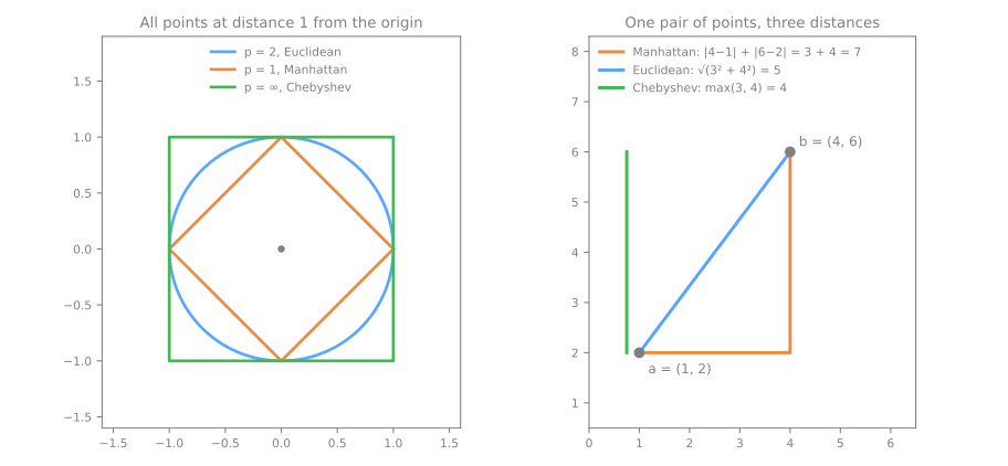
The left panel shows what each distance calls "a neighborhood": the set of points at distance 1 is a diamond, a circle or a square. Squaring makes the Euclidean distance sensitive to one large difference in a single feature. Manhattan adds differences without squaring them, so no single feature dominates as easily. Chebyshev looks only at the worst feature. In scikit-learn: KNeighborsClassifier(p=1) or metric='manhattan', p=2 (the default), metric='chebyshev'.
Two other distances you will meet:
- Cosine distance (\(1 - \cos\theta\)) compares the direction of two vectors and ignores their length. The vectors \((1, 1, 0)\) and \((10, 10, 0)\) are 12.7 apart in Euclidean distance but at cosine distance 0: the same "topic", one of them just longer. That is what you want for word counts and embeddings (Text Representation), where a long document should not be far from a short one about the same subject. Use
metric='cosine'. - Hamming distance counts the positions where two binary vectors differ. Nominal categories must be one-hot encoded first: coding
red, green, blueas 0, 1, 2 would make red "closer" to green than to blue, a fictitious distance.
In short, the choice depends on the kind of data:
| kind of data | distance | why |
|---|---|---|
| numeric features, already scaled | Euclidean (the default) | the straight line; works well when every feature matters |
| numeric features with large, isolated differences | Manhattan | adds without squaring: a single feature dominates less |
| word counts, TF-IDF, embeddings | cosine | compares direction and ignores length |
| binary vectors (one-hot, presence/absence) | Hamming | counts the positions where the vectors differ |
When in doubt, treat the distance as a hyperparameter and compare the options on validation, as you do with \(k\).
7. Ties, weighted votes and predict_proba
Stage 2. With two classes, an odd \(k\) can never produce a tied vote. With an even \(k\) it can, and scikit-learn does not break the tie by distance: it returns the class that comes first in classes_. In the subscriber example with \(k = 2\), Ana (yes) and Bruno (no) tie, and the prediction is "not liked" (class 0) even though the closest neighbor liked the series (see the next block). With three or more classes an odd \(k\) no longer guarantees anything (5 votes can split 2–2–1). Distance ties (two training points at exactly the same distance from the query, competing for the last place) are resolved by the order of the rows in the training data.
With weights='distance', each neighbor votes with weight \(1/d\), so closer neighbors count more. Redo \(k = 3\) for the new subscriber by hand: Ana weighs \(1/1 = 1.000\), Bruno \(1/2.236 = 0.447\), Carla \(1/2.828 = 0.354\). "Liked" gets 1.000, "not liked" gets \(0.447 + 0.354 = 0.801\), and
X_u, y_u = users[['action', 'docs']], users['liked']
for k in [2, 3]:
    for w in ['uniform', 'distance']:
        m = KNeighborsClassifier(n_neighbors=k, weights=w).fit(X_u, y_u)
        print(f"k={k} {w:8s} predict {m.predict(new)[0]}   P(liked) = {m.predict_proba(new)[0, 1]:.3f}")
k=2 uniform  predict 0   P(liked) = 0.500
k=2 distance predict 1   P(liked) = 0.691
k=3 uniform  predict 0   P(liked) = 0.333
k=3 distance predict 1   P(liked) = 0.555
Weighting flips both answers: Ana is much closer than Bruno and Carla, and now that counts. It also removes the \(k = 2\) tie (\(1/(1 + 0.447) = 0.691\)). Distance weighting makes k-NN less sensitive to the exact choice of \(k\), because far neighbors count little; treat weights as a second hyperparameter and choose it on validation too.
With uniform weights, predict_proba is a fraction of \(k\) neighbors, so it can only take the \(k + 1\) values \(0, 1/k, 2/k, \ldots, 1\):
for k in [5, 15, 73]:
    proba = KNeighborsClassifier(n_neighbors=k).fit(X_train, y_train).predict_proba(X_val)[:, 1]
    print(f"k={k:2d}: {len(np.unique(proba)):2d} distinct probabilities, e.g. {np.unique(proba)[:4].round(3)}")
k= 5:  6 distinct probabilities, e.g. [0.  0.2 0.4 0.6]
k=15: 16 distinct probabilities, e.g. [0.    0.067 0.133 0.2  ]
k=73: 62 distinct probabilities, e.g. [0.    0.014 0.027 0.041]
With \(k = 5\), the 200 validation points share only 6 possible probabilities. These are coarse scores, not the smooth output of a sigmoid. Keep it in mind for the next lessons, where metrics and ROC curves move a decision threshold across the scores: with 5-NN there are only 6 places to put it.
8. The curse of dimensionality
Stage 3. k-NN rests on one premise: near means similar. In many dimensions that premise breaks, in two measurable ways. (The dimensionality reduction lesson has a simulator of the first one.)
Distances concentrate. Scatter 1,000 random points in the unit cube, drop 100 query points, and compare each query's nearest and farthest neighbors (the median over the 100 queries describes a typical one):
for d in [2, 10, 100, 1000]:
    rng = np.random.default_rng(d)
    P = rng.uniform(size=(1000, d))                     # 1000 random points in the unit cube
    Q = rng.uniform(size=(100, d))                      # 100 query points
    D = pairwise_distances(Q, P)                        # 100 x 1000 distances
    near, far = D.min(axis=1), D.max(axis=1)            # for each query
    print(f"d={d:4d}  nearest {np.median(near):6.3f}  farthest {np.median(far):6.3f}  "
          f"(far - near)/near = {np.median((far - near) / near):6.2f}")   # typical query
d=   2  nearest  0.014  farthest  1.044  (far - near)/near =  71.21
d=  10  nearest  0.505  farthest  1.894  (far - near)/near =   2.69
d= 100  nearest  3.311  farthest  4.755  (far - near)/near =   0.44
d=1000  nearest 12.188  farthest 13.611  (far - near)/near =   0.12
In 2 dimensions a typical query has its nearest point at 0.014 and its farthest at 1.044: the gap between them is 71 times the nearest distance, so "nearest" singles out something meaningful. In 1,000 dimensions the nearest point is 12.2 away and the farthest 13.6, a gap of only 12%. Every point is roughly equally far, and the \(k\) "nearest" are barely nearer than the rest. Beyer et al. (1999) proved that, as \(d\) grows, this happens for a broad class of data distributions, not only uniform noise. The left panel of the figure below draws the same ratio for more values of \(d\).
Irrelevant features drown the useful ones. Real data does not have 1,000 dimensions of signal, but it often has many columns that carry none. Append pure-noise columns to the 13 wine features and compare k-NN with logistic regression:
from sklearn.linear_model import LogisticRegression

rng = np.random.default_rng(0)
Xw, yw = wine.data.to_numpy(), wine.target.to_numpy()
print("noise cols   k-NN   logistic")
for n_noise in [0, 10, 100, 1000]:
    Xn = np.hstack([Xw, rng.normal(size=(len(Xw), n_noise))])   # append pure-noise columns
    a, b, c, d = train_test_split(Xn, yw, test_size=0.3, stratify=yw, random_state=0)
    knn_acc = make_pipeline(StandardScaler(), KNeighborsClassifier(5)).fit(a, c).score(b, d)
    log_acc = make_pipeline(StandardScaler(), LogisticRegression(max_iter=2000)).fit(a, c).score(b, d)
    print(f"{n_noise:10d}   {knn_acc:.3f}  {log_acc:.3f}")
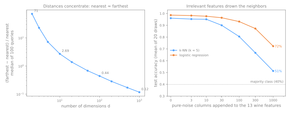
One split is noisy (logistic regression happens to lose 5.6 points at 10 noise columns), so the right panel averages 20 draws of noise and split. The pattern is clear: with 100 noise columns k-NN drops to 80% on average, with 1,000 to 51%, barely above the 40% of always answering the majority cultivar. The reason is in the formula. A Euclidean distance adds one squared difference per column, and every column counts the same. After standardization, 1,000 noise columns contribute about 77 times more to the distance than the 13 real ones, so the neighbors are chosen by noise. Logistic regression learns a weight per column and can push the noise weights toward zero, helped here by scikit-learn's default L2 penalty (the one the logistic regression lesson switched off with C=np.inf), which keeps weights small; it degrades too, but much later.
Remedies: keep only relevant features (feature selection, domain knowledge), compress with PCA before k-NN, or learn the distance itself (metric learning). k-NN shines in few, meaningful dimensions with plenty of data.
9. Cost at prediction time
As section 2 anticipated, k-NN is a lazy learner: fit postpones all the work to prediction time. Timing it would give numbers that depend on your machine, so count instead. The distance below is the ordinary Euclidean one, with a counter added:
import numpy as np

calls = 0
def euclidean(a, b):                     # the usual distance, plus a counter
    global calls
    calls += 1
    return np.sqrt(((a - b) ** 2).sum())

rng_demo = np.random.default_rng(0)
X_big = rng_demo.uniform(size=(2000, 2)); y_big = (X_big[:, 0] > 0.5).astype(int)
queries = rng_demo.uniform(size=(20, 2))

knn = KNeighborsClassifier(n_neighbors=5, algorithm='brute', metric=euclidean)
knn.fit(X_big, y_big);   print(f"fit:     {calls:6d} distances")
calls = 0
knn.predict(queries);    print(f"predict: {calls:6d} distances for {len(queries)} queries")
Fitting on 2,000 rows computed nothing. Each of the 20 predictions computed 2,000 distances, one per stored row. The cost of a prediction is \(O(n \cdot d)\): double the training set and every prediction costs twice as much. That is the opposite profile from logistic regression, which does all its work in fit and then predicts almost for free.
Brute force compares the query with every stored row. Search trees (algorithm='kd_tree' or 'ball_tree') organize the training points into nested regions at fit time, so a query can skip whole regions that are provably too far. With the counting distance from before:
for d in [2, 10, 50]:
    Xd = rng.uniform(size=(2000, d)); yd = (Xd[:, 0] > 0.5).astype(int)
    Qd = rng.uniform(size=(20, d))
    for algo in ['brute', 'ball_tree']:
        knn = KNeighborsClassifier(n_neighbors=5, algorithm=algo, metric=euclidean).fit(Xd, yd)
        calls = 0
        knn.predict(Qd)
        print(f"d={d:2d} {algo:9s} {calls / len(Qd):6.0f} distances per query")
d= 2 brute       2000 distances per query
d= 2 ball_tree    118 distances per query
d=10 brute       2000 distances per query
d=10 ball_tree   2124 distances per query
d=50 brute       2000 distances per query
d=50 ball_tree   2127 distances per query
In 2 dimensions the ball tree finds the 5 nearest of 2,000 points with 118 distance computations instead of 2,000, 17 times fewer. In 10 and 50 dimensions it computes more than brute force: when all distances are similar (the concentration above), no region can be ruled out, and the tree adds its own overhead. The default algorithm='auto' picks a method from the shape of the data.
For millions of rows in hundreds of dimensions (image or text embeddings), exact search is too slow, and systems use approximate nearest neighbors (graph indexes such as HNSW, libraries such as FAISS): they return almost the \(k\) nearest, orders of magnitude faster. This "find the nearest embeddings" operation is the heart of the vector databases behind retrieval-augmented LLM systems (The Frontier): a 1951 idea serving 2020s systems.
10. k-NN vs logistic regression
Stage 4. Two curved problems, same hold-out protocol, default settings for both models (both features are already on the same scale):
from sklearn.datasets import make_circles

for name, (Xs, ys) in [('moons', (X, y)),
                       ('circles', make_circles(n_samples=1000, noise=0.1, factor=0.5, random_state=0))]:
    a, b, c, d = train_test_split(Xs, ys, test_size=0.3, stratify=ys, random_state=0)
    log_acc = LogisticRegression().fit(a, c).score(b, d)
    knn_acc = KNeighborsClassifier(n_neighbors=15).fit(a, c).score(b, d)
    print(f"{name:8s} logistic {log_acc:.3f}   k-NN {knn_acc:.3f}")
On the moons, a straight line already separates most points, and k-NN gains 6.4 points by bending around the tips. On the circles (one class inside a ring of the other) no straight line helps at all: logistic regression scores 49.3%, a coin flip, while k-NN scores 99.3%. Logistic regression could get there too, with hand-made features such as \(x_1^2 + x_2^2\) (polynomial features); k-NN needs no feature engineering to follow a curve.
Section 8 showed the reverse: with many irrelevant columns, logistic regression wins by 11 points at 100 noise columns (90.7% vs 79.6%) and 13 points at 1,000 (68.5% vs 55.6%), because it can learn to ignore a column and k-NN cannot. Neither model is better in general:
| situation | favors |
|---|---|
| curved boundary, few features, plenty of rows | k-NN |
| many features, some of them irrelevant | logistic regression |
| predictions must be fast, or the training set is huge | logistic regression |
| you must explain the effect of each feature | logistic regression (coefficients, odds) |
| you must explain a single decision | k-NN ("these are the most similar cases") |
11. k-NN for regression
KNeighborsRegressor works the same way but predicts the average of the \(k\) neighbors' target values (weighted by \(1/d\) with weights='distance'). Everything above carries over: scale the features, choose \(k\) on validation, beware of high dimensions. One extra limit: an average of neighbors can never predict outside the range of the training targets, so k-NN cannot extrapolate a trend.
12. Practical profile
| Strengths | nothing to fit; any boundary shape; naturally multi-class; one intuitive hyperparameter; a strong, easy-to-explain baseline ("similar cases were…") |
| Weaknesses | prediction costs \(O(n \cdot d)\) per query (trees help only in low dimensions); memory = the whole training set; needs scaling; hurt by irrelevant features and high dimension; coarse probabilities (\(k + 1\) values) |
| Knobs | n_neighbors (choose on validation), weights ('uniform' / 'distance'), metric / p, algorithm (speed only) |
| Classic uses | recommendations ("users like you"), image and document retrieval, anomaly detection (distance to the \(k\)-th neighbor), imputation (KNNImputer), semantic search over embeddings |
A theoretical footnote from Cover & Hart (1967): with unlimited data, the error of 1-NN is at most twice the smallest error any classifier can achieve on the problem. It is a remarkable guarantee for a method that learns nothing, and the "unlimited data" part is exactly what the curse of dimensionality takes away.
Advanced lab — handwritten digits
The digits dataset holds 1,797 handwritten digits as 8×8 images; each pixel is a feature, 64 in total. Here you can see the neighbors and find out what the distance means by "similar", and what it does not. Steps 6 to 8 revisit three themes of this part: when scaling does not help, the distance as the limit of the model, and the curse of dimensionality.
How to run this lab in class (about 25 min, in pairs)
- Use the same Colab notebook as the fundamental lab and go to step 6 (Passo 6). Nothing to download.
- Steps 6 to 8 use the libraries imported in steps 1 to 3. If the Colab session is new (or has expired), click the step 6 cell and use Runtime → Run before (Ctrl+F8) before going on.
- Same routine: Predict before running, compare with the page, and try the Simulations before opening the solution.
- Suggested pace: steps 6 and 7 in 12 min; step 8 in 8 min; wrap-up in 5 min.
Step 6 — digits: a dataset where the pixels are the features
Predict. In an 8×8 image, the 64 pixels already share one unit (ink, from 0 to 16). Will standardizing help, hurt, or change nothing? And which digits do you expect k-NN to confuse?
from sklearn.datasets import load_digits

digits = load_digits()
Xd, yd = digits.data, digits.target          # 1797 images of 8x8 pixels, each pixel 0 to 16
Xd_train, Xd_test, yd_train, yd_test = train_test_split(Xd, yd, test_size=0.25,
                                                        stratify=yd, random_state=0)
print(Xd.shape, len(Xd_train), len(Xd_test))

knn_d = KNeighborsClassifier(n_neighbors=3).fit(Xd_train, yd_train)
pred = knn_d.predict(Xd_test)
scaled = make_pipeline(StandardScaler(), KNeighborsClassifier(n_neighbors=3)).fit(Xd_train, yd_train)
print(f"baseline           {DummyClassifier().fit(Xd_train, yd_train).score(Xd_test, yd_test):.3f}")
print(f"3-NN, raw pixels   {(pred == yd_test).mean():.3f}")
print(f"3-NN, standardized {scaled.score(Xd_test, yd_test):.3f}")

wrong = np.flatnonzero(pred != yd_test)
print(f"{len(wrong)} of {len(yd_test)} test digits misclassified")
print(pd.crosstab(pd.Series(yd_test, name='true'), pd.Series(pred, name='predicted')))
(1797, 64) 1347 450
baseline           0.102
3-NN, raw pixels   0.987
3-NN, standardized 0.982
6 of 450 test digits misclassified
predicted   0   1   2   3   4   5   6   7   8   9
true
0          45   0   0   0   0   0   0   0   0   0
1           0  46   0   0   0   0   0   0   0   0
2           0   0  44   0   0   0   0   0   0   0
3           0   0   0  45   0   0   0   1   0   0
4           0   0   0   0  44   0   0   0   0   1
5           0   0   0   0   0  46   0   0   0   0
6           0   0   0   0   0   0  45   0   0   0
7           0   0   0   0   0   0   0  45   0   0
8           0   1   0   1   0   0   0   0  41   0
9           0   0   0   2   0   0   0   0   0  43
Each image is flattened into 64 numbers, the ink intensity of each pixel, and the distance between two images is the Euclidean distance between those vectors. With 10 balanced classes the baseline is 10.2%; 3-NN gets 98.7% of the 450 test digits right. Here scaling does not help (98.2%): all 64 features already share one unit, and standardizing gives the nearly blank border pixels as much say as the pixels that carry the strokes. "Always scale" really means "never let units decide by accident".
In the table, rows are the true digit and columns the prediction; the diagonal holds the correct answers. The 6 mistakes are not random: two 9s were read as 3, and two 8s were read as 1 and as 3, pairs of digits that share strokes. This table is the confusion matrix; the next lesson builds a whole family of metrics out of it.
Step 7 — look at the neighbors
Predict. For a 9 that the model read as a 3, what images do you expect to find among its 5 nearest neighbors?
fig, axes = plt.subplots(2, 6, figsize=(8, 3.3))
for row, i in zip(axes, [0, wrong[0]]):                     # one right, one wrong
    dist, idx = knn_d.kneighbors(Xd_test[[i]], n_neighbors=5)
    print(f"test #{i}: true {yd_test[i]}, predicted {pred[i]} · neighbors {yd_train[idx[0]]} "
          f"at distances {dist[0].round(1)}")
    row[0].imshow(Xd_test[i].reshape(8, 8), cmap='gray_r')
    row[0].set_title(f"true {yd_test[i]}, pred {pred[i]}")
    for ax, j, d in zip(row[1:], idx[0], dist[0]):
        ax.imshow(Xd_train[j].reshape(8, 8), cmap='gray_r')
        ax.set_title(f"{yd_train[j]} (d={d:.1f})")
    for ax in row:
        ax.axis('off')
plt.tight_layout()
plt.show()
test #0: true 2, predicted 2 · neighbors [2 2 2 2 2] at distances [20.3 20.6 20.7 24.  25.1]
test #32: true 9, predicted 3 · neighbors [3 3 3 9 9] at distances [21.9 26.5 27.8 28.2 29.4]
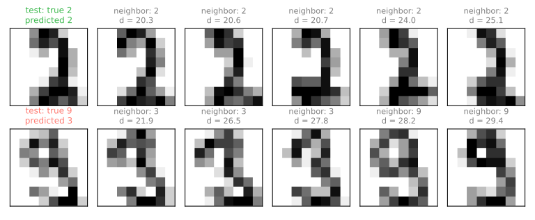
This is k-NN's great advantage: every prediction comes with its evidence. The 2 is surrounded by 2s. The misread 9 is drawn with a thin, open loop; its three closest training images are 3s (at 21.9, 26.5 and 27.8), and the first 9s only arrive in 4th and 5th place (28.2 and 29.4). With \(k = 5\) the vote would still be 3 against 2. No weight or coefficient to interpret: you can show a user the five most similar cases and let them judge.
Simulation: shift a digit by one pixel. Take the test 2 #0 and shift the image one column to the right (the column that comes in is blank). How far is the shifted image from the original? Compare with the distance of the neighbors above (20.3). What does 3-NN predict for it? Then shift all test images by 1 and 2 pixels, both ways, and measure the accuracy.
Solution
def shift(X, dx):
    """Shift 8x8 images by dx columns (dx > 0: to the right); what comes in is blank."""
    imgs = X.reshape(-1, 8, 8)
    out = np.zeros_like(imgs)
    if dx > 0:
        out[:, :, dx:] = imgs[:, :, :-dx]
    elif dx < 0:
        out[:, :, :dx] = imgs[:, :, -dx:]
    else:
        out = imgs.copy()
    return out.reshape(len(X), 64)

moved = shift(Xd_test[[0]], 1)
dist, idx = knn_d.kneighbors(moved)
print(f"distance to its own original image: {np.linalg.norm(moved - Xd_test[[0]]):.1f}")
print(f"prediction: {knn_d.predict(moved)[0]} · neighbors {yd_train[idx[0]]} at distances {dist[0].round(1)}")
for dx in [-2, -1, 0, 1, 2]:
    print(f"shift {dx:+d}: accuracy {knn_d.score(shift(Xd_test, dx), yd_test):.3f}")
distance to its own original image: 50.7
prediction: 0 · neighbors [9 0 0] at distances [50.4 50.4 50.4]
shift -2: accuracy 0.162
shift -1: accuracy 0.598
shift +0: accuracy 0.987
shift +1: accuracy 0.604
shift +2: accuracy 0.133
To our eyes, the shifted 2 is the same 2. To the distance, it is 50.7 away from its own original image, more than twice the distance to other 2s written by other people (20.3). The distance compares pixel with pixel: a stroke that moved one column lands on pixels that used to be blank, and the image becomes "something else". Its nearest neighbors are all at 50.4, almost as far as its own original: nothing in the training set looks like a shifted 2, and 3-NN predicts 0. On the whole test set, shifting by one pixel drops accuracy from 98.7% to about 60%; by two pixels, to about 15%, close to guessing. k-NN is only as good as the distance you give it. This one knows nothing about shape; the remedies are to add shifted copies of the images to the training set (Your turn) or to use features that do not change with a shift, like the ones neural networks learn.
Step 8 — add noise features
Predict. Add to the 64 real columns some columns of pure noise, in the same 0–16 range. With 64 noise columns (as many as the real ones), does accuracy fall a lot or a little? And with 1,024?
rng = np.random.default_rng(0)
for n_noise in [0, 64, 256, 1024]:
    noise = rng.uniform(0, 16, size=(len(Xd), n_noise))      # fake "pixels", same range as real ones
    Xn = np.hstack([Xd, noise])
    a, b, c, d = train_test_split(Xn, yd, test_size=0.25, stratify=yd, random_state=0)
    acc = KNeighborsClassifier(n_neighbors=3).fit(a, c).score(b, d)
    print(f"{n_noise:5d} noise columns ({Xn.shape[1]:4d} in total): accuracy {acc:.3f}")
    0 noise columns (  64 in total): accuracy 0.987
   64 noise columns ( 128 in total): accuracy 0.960
  256 noise columns ( 320 in total): accuracy 0.842
 1024 noise columns (1088 in total): accuracy 0.582
The noise columns look like pixels but carry no information. With as many fake pixels as real ones, accuracy drops from 98.7% to 96.0%; with 1,024 of them, to 58.2%. The images have not changed and the 64 real pixels are all still there; they are simply outvoted inside the distance, where every column counts the same. This is the curse of dimensionality in its most practical form: before blaming k-NN, ask how many of your columns actually matter.
Simulation: the size of the noise. Keep 1,024 noise columns, but draw them in smaller ranges: 0 to 16, 0 to 4 and 0 to 1. For each range, measure the accuracy of 3-NN without scaling and with StandardScaler in a pipeline. What hurts k-NN: the number of noise columns, or how much they add to the distance?
Solution
rng = np.random.default_rng(1)
for high in [16, 4, 1]:
    noise = rng.uniform(0, high, size=(len(Xd), 1024))     # 1024 noise columns, from 0 to high
    a, b, c, d = train_test_split(np.hstack([Xd, noise]), yd, test_size=0.25, stratify=yd, random_state=0)
    raw = KNeighborsClassifier(n_neighbors=3).fit(a, c).score(b, d)
    std = make_pipeline(StandardScaler(), KNeighborsClassifier(n_neighbors=3)).fit(a, c).score(b, d)
    print(f"noise from 0 to {high:2d}: raw {raw:.3f} · standardized {std:.3f}")
noise from 0 to 16: raw 0.544 · standardized 0.429
noise from 0 to  4: raw 0.982 · standardized 0.424
noise from 0 to  1: raw 0.987 · standardized 0.462
Without scaling, the same 1,024 columns barely hurt when they are small: with noise from 0 to 1, 3-NN is back to the 98.7% of the clean images, because each fake column adds very little to the distance and the real pixels decide. (With noise from 0 to 16 it gets 54.4%, not the 58.2% of step 8, because the noise drawn is different.) What hurts is how much the useless columns weigh in the distance, not how many there are. StandardScaler undoes that: it gives every column the same weight, useless ones included, and accuracy stays below 50% in all three ranges. Scaling is needed so that units do not decide by accident, but it does not separate useful columns from useless ones. That is your job: choose the features before measuring distances.
To close the class. One sentence each: (1) why was a 2 shifted by one pixel read as a 0? (2) Why did standardizing help on the wines and not on the digits? (3) In step 8, what hurt k-NN: the number of noise columns, or how much they weigh in the distance?
Your turn (advanced)
For homework, with more time:
- Weights. Repeat step 5 with
KNeighborsClassifier(n_neighbors=k, weights='distance'). Does training accuracy stay at 1.000 for every \(k\)? Why? (Hint: what is the weight of a neighbor at distance 0?) - Choose \(k\) for the digits. Step 6 used \(k = 3\) without justification. Carve a validation split out of
Xd_train, score odd \(k\) from 1 to 15 withmetric='euclidean'and withmetric='manhattan', pick the best pair, and only then measure the test set once. - Teach it the shift. Add to the training set copies of each image shifted one pixel to the left and to the right (use the
shiftfunction of the step 7 simulation; the labels repeat). Measure the accuracy on the shifted test images again. How much comes back? What does it cost, in stored rows and in distances per prediction? - Rescue with PCA. On the version with 1,024 noise columns from 0 to 16, put
PCA(n_components=30)before k-NN in a pipeline. How much of the lost accuracy comes back? Why might PCA separate the real pixels from the noise here? (Dimensionality Reduction) - Regression. With
load_diabetes(return_X_y=True), compareKNeighborsRegressor(scaled, \(k\) chosen on a validation split) withLinearRegressionon a hold-out, using \(R^2\). Which one wins, and does it match what the curse of dimensionality section would predict with 10 features and 442 rows?
References
- Fix, E.; Hodges, J. L. "Discriminatory Analysis. Nonparametric Discrimination: Consistency Properties." Report 4, USAF School of Aviation Medicine (1951); reprinted in International Statistical Review 57 (1989). DOI
- Cover, T.; Hart, P. "Nearest Neighbor Pattern Classification." IEEE Trans. Inf. Theory 13 (1967) — the "at most twice the Bayes error" bound. DOI
- Beyer, K.; Goldstein, J.; Ramakrishnan, R.; Shaft, U. "When Is 'Nearest Neighbor' Meaningful?" Database Theory — ICDT'99, LNCS 1540, Springer (1999): 217–235 — distance concentration in high dimensions. DOI
Quiz
The quiz covers the fundamental approach.