The path of this part
- Choose the distanceMinkowski, cosine, Hamming: by the kind of data
- How the vote countsties, 1/d weights, a coarse
predict_proba - Where it breaksthe curse of dimensionality; the cost of predicting
- When to use itagainst logistic regression; regression; practical profile
The Minkowski family
\[ d_p(a, b) = \Big( \sum_{j=1}^{d} \lvert a_j - b_j \rvert^p \Big)^{1/p} \]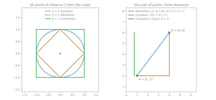
\(a = (1, 2)\), \(b = (4, 6)\): differences 3 and 4.
| \(p = 1\) Manhattan | \(3 + 4 = 7\) |
| \(p = 2\) Euclidean | \(\sqrt{9 + 16} = 5\) |
| \(p = \infty\) Chebyshev | \(\max(3, 4) = 4\) |
Squaring makes the Euclidean distance sensitive to one large difference in a single feature.
Choose the distance by the kind of data
| kind of data | distance | why |
|---|---|---|
| numeric, scaled | Euclidean | the straight line; the default |
| large, isolated differences | Manhattan | a single feature dominates less |
| text, TF-IDF, embeddings | cosine | compares direction, ignores length |
| binary, one-hot | Hamming | counts differing positions |
Ties
- With two classes, an odd \(k\) never ties; an even \(k\) can.
- scikit-learn does not break ties by distance: it returns the class that comes first in
classes_. - Subscribers with \(k = 2\): Ana (yes, \(d = 1\)) × Bruno (no, \(d = 2.24\)) → predicts "not liked", even though the closest one liked it.
- With 3 or more classes an odd \(k\) guarantees nothing: 5 votes can split 2–2–1.
Weighted votes: weight \(1/d\)
\(k = 3\) for the new subscriber:
- Ana: \(1/1 = 1.000\) → liked
- Bruno: \(1/2.236 = 0.447\) → no
- Carla: \(1/2.828 = 0.354\) → no
| \(k\) | weights | predicts | P(liked) |
|---|---|---|---|
| 2 | uniform | 0 | 0.500 |
| 2 | distance | 1 | 0.691 |
| 3 | uniform | 0 | 0.333 |
| 3 | distance | 1 | 0.555 |
Weighting flips both answers and removes the tie. weights is a second hyperparameter: choose it on validation.
predict_proba is coarse
With uniform weights it is a fraction of \(k\) neighbors: only \(k + 1\) possible values, \(0, 1/k, \ldots, 1\).
| \(k\) | distinct probabilities on the 200 validation points |
|---|---|
| 5 | 6 |
| 15 | 16 |
| 73 | 62 |
Curse 1: distances concentrate
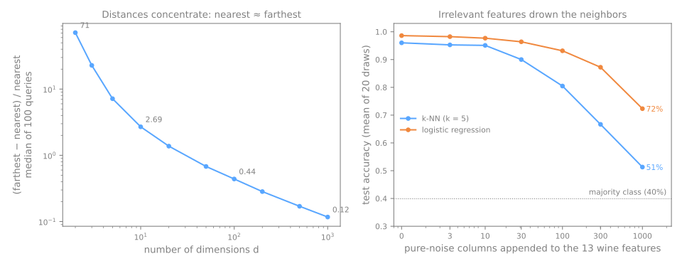
1,000 random points in the unit cube, 100 queries; median per query:
| dimensions | nearest | farthest | (far − near)/near |
|---|---|---|---|
| 2 | 0.014 | 1.044 | 71.21 |
| 10 | 0.505 | 1.894 | 2.69 |
| 100 | 3.311 | 4.755 | 0.44 |
| 1,000 | 12.188 | 13.611 | 0.12 |
Curse 2: irrelevant columns drown the useful ones
Wines (13 features) + pure-noise columns:
| noise | k-NN | logistic |
|---|---|---|
| 0 | 0.963 | 1.000 |
| 10 | 0.963 | 0.944 |
| 100 | 0.796 | 0.907 |
| 1,000 | 0.556 | 0.685 |
Cost: the lazy learner, measured
fit on 2,000 rows
predict of 20 queries
cost per query
Search trees (ball_tree) skip regions that are too far:
| dimensions | brute force | ball tree |
|---|---|---|
| 2 | 2,000 | 118 |
| 10 | 2,000 | 2,124 |
| 50 | 2,000 | 2,127 |
At scale: approximate neighbors
- Millions of rows in hundreds of dimensions (image or text embeddings): exact search is too slow.
- Approximate nearest neighbors (graph indexes such as HNSW, libraries such as FAISS) return almost the \(k\) nearest, orders of magnitude faster.
- That is the heart of the vector databases behind retrieval-augmented LLM systems (RAG).
k-NN vs logistic regression
| data | logistic | k-NN (\(k = 15\)) |
|---|---|---|
| moons | 0.833 | 0.897 |
| circles | 0.493 | 0.993 |
No straight line separates a disc from the ring around it.
| situation | favors |
|---|---|
| curved boundary, few features, plenty of rows | k-NN |
| many features, some irrelevant | logistic |
| fast predictions, huge training set | logistic |
| explain the effect of each feature | logistic |
| explain a single decision | k-NN |
k-NN for regression, and a theoretical guarantee
KNeighborsRegressor
- predicts the average target of the \(k\) neighbors (weighted by \(1/d\) with
weights='distance'); - same care: scale, choose \(k\) on validation, avoid high dimension;
- an average never leaves the range of the training targets: it cannot extrapolate a trend.
Cover & Hart (1967)
With unlimited data, the error of 1-NN is at most twice the smallest error achievable on the problem.
The "unlimited data" part is exactly what the curse of dimensionality takes away.
Practical profile
Strengths
- nothing to fit; any boundary shape
- naturally multi-class
- a strong, easy-to-explain baseline
- uses: recommendation, semantic search, anomalies,
KNNImputer
Weaknesses
- prediction costs \(O(n \cdot d)\); memory = the whole training set
- needs scaling
- hurt by irrelevant features and high dimension
- coarse probabilities (\(k + 1\) values)
Hyperparameters: n_neighbors, weights, metric/p; algorithm only changes speed.
Handwritten digits: steps 6 to 8
- Same Colab notebook, from step 6 (Passo 6). New session? Runtime → Run before.
- 8×8 images: the 64 pixels are the features, all in one unit.
- Step 7: look at the neighbors of a 9 read as a 3; simulation: shift a digit by one pixel.
- Step 8: noise columns; simulation: the size of the noise.
Pace: steps 6 and 7 in 12 min; step 8 in 8 min; wrap-up in 5 min.