Two ways to use the training data
Logistic regression
- reads the whole training set
- sums it up in \(d + 1\) numbers
- draws a straight line
- throws the rows away
k-NN
- keeps every row
- for a new point, finds the \(k\) most similar
- they vote
- the boundary takes any shape the data suggests
The path of this part
- Neighbors votedistance to every row; the k nearest vote;
fitonly stores - Scale firstunits decide the distance; the scaler goes inside a pipeline
- Choose k, test oncebias and variance; validation chooses, the test confirms
A problem: will they like the series?
- A streaming service is about to recommend a series that mixes action and documentary.
- For 10 subscribers who have watched it, we know their weekly hours of action films and of documentaries, and whether they liked it.
- A new subscriber watches 4 h of action and 4 h of documentaries.
"Similar" becomes a number: the Euclidean distance to the new subscriber.
\[ d = \sqrt{(\text{action} - 4)^2 + (\text{docs} - 4)^2} \]First: measure the distance to each one
| rank | name | action | docs | liked? | \(d\) |
|---|---|---|---|---|---|
| 1 | Ana | 5 | 4 | yes | 1.000 |
| 2 | Bruno | 2 | 5 | no | 2.236 |
| 3 | Carla | 6 | 6 | no | 2.828 |
| 4 | Davi | 4 | 7 | yes | 3.000 |
| 5 | Elisa | 7 | 3 | yes | 3.162 |
| 6–10 | Felipe, Gabi, Hugo, Iara, João: from 3.606 to 5.831 | ||||
Ana: \(\sqrt{(5-4)^2 + (4-4)^2} = 1\). Sort from nearest to farthest.
Then: the \(k\) nearest vote
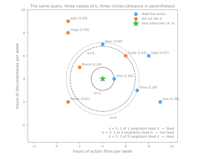
- \(k = 1\): Ana → liked (1/1)
- \(k = 3\): 1 yes × 2 no → not liked (1/3)
- \(k = 5\): 3 yes × 2 no → liked (3/5)
The algorithm in three steps
- compute the distance from the query \(x\) to every training point;
- keep the \(k\) closest, the neighborhood \(N_k(x)\);
- predict the most frequent class among them.
The "probability" of class \(c\) is just the fraction of neighbors in it:
\[ \hat{p}_c(x) = \frac{1}{k} \sum_{i \in N_k(x)} \mathbb{1}[y_i = c] \]In the example, predict_proba gives 1.000, 0.333 and 0.600 for \(k\) = 1, 3 and 5.
What fit stores
| logistic regression | k-NN | |
|---|---|---|
fit produces | \(d + 1\) numbers | a copy of the training table |
| boundary | a straight line (hyperplane) | any shape |
cost of fit | iterative optimization | almost none: store |
| cost of predicting | \(d\) multiplications | \(n\) distances |
| explains with | one coefficient per feature | "these are the most similar cases" |
Units decide the distance
A new travel-agency customer: R$ 5,000 per month, 25 years old. Will they buy the backpacking package?
| customer | income | age | bought? | raw \(d\) | standardized \(d\) |
|---|---|---|---|---|---|
| Rita | 5,200 | 61 | no | 203.2 | 2.57 |
| Otávio | 5,700 | 26 | yes | 700.0 | 0.32 |
- Raw: \(\sqrt{200^2 + 36^2} = 203.2\). The 36 years add only 3.2, because one year weighs as much as one real. 1-NN: Rita → no.
- Standardized (each feature ÷ its standard deviation): the nearest is Otávio → yes.
The same case, as a figure
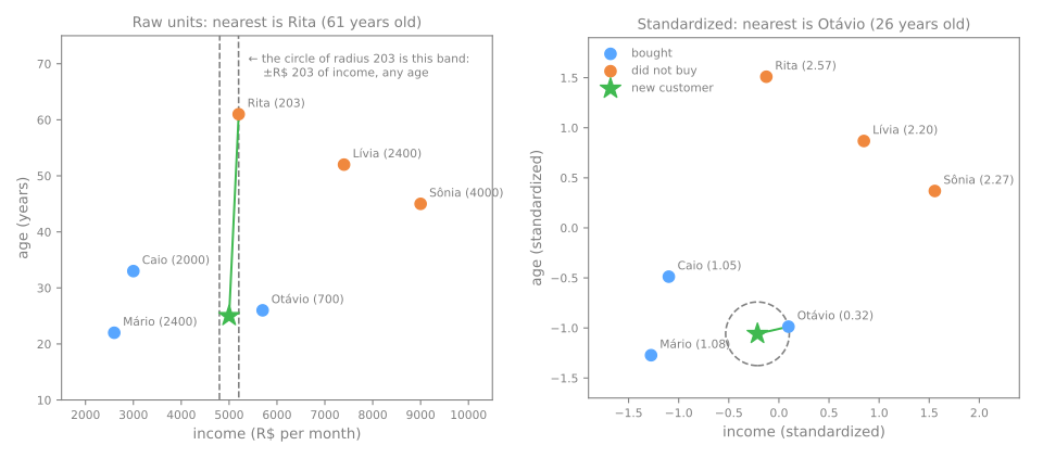
In raw units, a "circle" of radius 203 is a band R$ 203 wide on each side that contains every age.
On a real dataset: the wines
Standard deviation of the wine features:
| proline | 314.91 |
| magnesium | 14.28 |
| alcalinity_of_ash | 3.34 |
| color_intensity | 2.32 |
Test accuracy of 5-NN (54 wines):
| no scaling | 0.722 |
StandardScaler | 0.963 |
MinMaxScaler | 0.963 |
Rule: scale, always inside a pipeline
from sklearn.neighbors import KNeighborsClassifier
from sklearn.pipeline import make_pipeline
from sklearn.preprocessing import StandardScaler

knn = make_pipeline(StandardScaler(),
                    KNeighborsClassifier(n_neighbors=5))
knn.fit(X_train, y_train)
- the scaler learns means and standard deviations from training rows only;
- validation and test get the same transformation, without refitting;
- exception: features that already share one unit (the pixels of the advanced lab).
\(k\) is the complexity knob
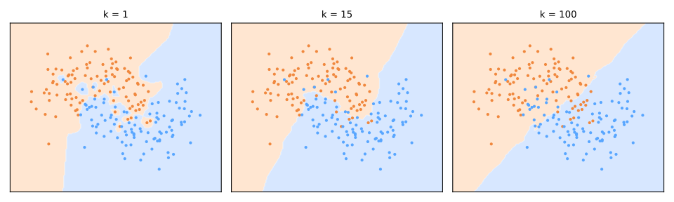
\(k = 1\): islands around each point (train 100%, validation 85.0%) · \(k = 15\): follows the moons (89.5%) · \(k = 451\): almost a straight line (76.5%)
Choose \(k\) on validation
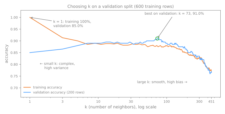
- 100% training accuracy at \(k = 1\) is by construction: each point is its own neighbor.
- Plateau: from \(k = 7\) to ~140, validation stays between 88.5% and 91.0%.
- Large \(k\): training and validation fall together → too simple.
The protocol: each split has a job
training · 600
the rows k-NN stores, and the ones that vote
validation · 200
chooses \(k\)
test · 200
measured once, at the end, after refitting on training + validation
Simulator: the vote of the neighbors
Predict. The ★ sits on the boundary. Sweep \(k\) from 1 to 25 without moving it: does its class stay the same? Then drag it through the overlap: which \(k\) flips more?
Summary: the k-NN recipe
- Pipeline with scaler + k-NN.
- Split before looking: training, validation, test.
- Sweep odd \(k\) on validation (with two classes, an odd \(k\) never ties).
- Refit on training + validation and measure the test set once.
Wines: steps 1 to 5
- Open the notebook on Colab (in Portuguese): nothing to download. Save a copy to your Drive to keep your answers.
- In each step, answer the Predict before running.
- Simulations: the unit of proline (step 3) and the vote changes with \(k\) (step 4).
- Compare with the output and the reading on the lesson page.
Pace: steps 1 to 3 in 15 min; steps 4 and 5 in 20 min.