Linear Regression

Linear regression is the oldest algorithm in this course. Legendre published least squares in 1805 to fit comet orbits, in an appendix titled Sur la Méthode des moindres quarrés, and Gauss claimed he had been using it since 1795 — but neither of them called it regression. That word arrived eighty years later, from a study of human height, and it described a phenomenon rather than a method. Two centuries on, the model remains the first thing to try on any continuous target: fast, interpretable, and a baseline that is embarrassingly hard to beat.

This lesson takes one idea and follows it all the way down: fit a line, look at what it got wrong, and use those errors to do better. The errors are the residuals; using them systematically is the gradient.

How this lesson is organized

The lesson has two approaches. Each has slides, text and a lab to do in class on Colab; the quiz at the end covers the fundamental one. Start with the fundamental approach: the advanced one builds on it.

Both labs use the same notebook on Colab, Regressão linear do zero (in Portuguese): the fundamental part runs from step 1 to 4 (the notebook's sections 1 to 4), the advanced part from step 5 to 10 (its sections 5 and 6). Everything runs in the browser; there is nothing to download.

Fundamental approach

One question drives this part: among all the lines that could be drawn through a cloud of points, which one is best, and how good is it? The answer is a rule (make the squared vertical errors as small as possible), two formulas that follow from it, and a habit: look at what the line got wrong. Everything is done first by hand, on five points, and then checked in Python.

This part follows one path in five stages, drawn below: 1. Galton's puzzle, where the word regression comes from; 2. the model, a prediction as a weighted sum of features; 3. least squares, the rule that picks the line; 4. residuals, what the line got wrong; 5. measuring quality, how to summarize those errors in one number. Each stage links to its section, and in the slides a strip at the bottom shows which stage you are in.

Fundamental approach slides

Click the slides and use the ← → arrows to navigate; F opens full screen and Esc shows every slide. Open the slides in a new tab

1. Where the name comes from

Stage 1. In 1886 Francis Galton published Regression toward Mediocrity in Hereditary Stature. He had collected the heights of 928 adult children and their parents, and he was looking for the strength of heredity. What he found puzzled him.

Very tall parents did have tall children — but on average, the children were closer to the population mean than their parents were. Very short parents had short children who were, again, closer to the middle. Galton first called this "reversion", then "regression toward mediocrity". The name stuck to the technique he used to measure it, which is why an algorithm about fitting lines carries a word that means "moving backwards".

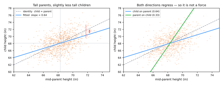
The left panel is the effect itself. The dashed line is identity — what the data would look like if children simply matched their parents. The fitted line is flatter. A mid-parent 3 inches above average produces a child predicted only about 2 inches above average. The red arrow is the gap, and that gap is the "regression".

The slope Galton reported was about \(2/3\), and it is worth seeing where that comes from:

Correlation and slope are not the same number. The slope carries the units; the correlation is what is left after you strip them out. They coincide only when both variables are measured in the same spread — which is exactly the situation the simulator below puts you in, so you can watch the geometry without the unit bookkeeping.

One figure in that calculation deserves a second look: why do children (2.52) vary more than mid-parents (1.80)? Not because parents are a more uniform group. Mid-parent is the average of two people, and averaging shrinks spread: two individuals at \(s \approx 2.5\) average to \(2.5/\sqrt{2} \approx 1.77\), which is essentially the 1.80 Galton reported. The asymmetry is an artifact of how the \(x\) variable was constructed, not a fact about heredity — and noticing that is the same habit of mind the rest of this section is about.

2. The model

Stage 2. Predict a continuous target as a weighted sum of features:

• \(w_j\) is the change in \(\hat{y}\) per unit change in \(x_j\), holding the other features fixed;
• \(w_0\) (intercept, or bias) is the prediction when every feature is zero.

In matrix form, with a leading column of 1s absorbed into \(X\): \(\hat{y} = Xw\).

Reading the coefficients

Back to the first bullet: the four words holding the other features fixed carry more weight than they look. Read this fitted model for apartment prices:

3200 does not mean "bigger apartments cost R$ 3200 more per m² in this city". It means: among apartments of the same age, one extra m² is associated with R$ 3200 more. If area and age happen to be correlated in your data — say newer buildings are larger — then the raw relationship between area and price mixes both effects, and the coefficient deliberately separates them.

3. Why not just invert \(X\)?

Written as \(\hat{y} = Xw\), the natural reflex is \(w = X^{-1}y\). It does not work, and seeing exactly why is the fastest route into what least squares is actually doing.

Take three observations and two parameters:

First obstacle: \(X\) is not square. It is \(3 \times 2\), and only square matrices have inverses. In general \(X\) is \(n \times d\) with \(n \gg d\) — thousands of rows, a handful of columns.

Second obstacle, and the real one: there is no exact solution anyway. \(y = Xw\) is three equations in two unknowns — an overdetermined system. An exact \(w\) exists only if \(y\) happens to lie in the column space of \(X\), and here it does not:

Appending \(y\) raised the rank, so \(y\) points somewhere the columns of \(X\) cannot reach. No \(w\) whatsoever satisfies \(Xw = y\). That is not bad luck — it is the normal situation, and it is the whole reason regression exists. If an exact solution did exist, every residual would be zero and the line would pass through every point.

What we do instead

Since \(y\) is out of reach, settle for the reachable point closest to it — minimize \(\lVert y - Xw\rVert^2\). Setting the gradient to zero gives the normal equations, and the trick is what happens to the shapes:

\(X^\top X\) is \(2 \times 2\) — square, and invertible whenever \(X\) has full column rank. We never invert \(X\); we invert \(X^\top X\). Two equations, small enough to solve on paper:

The fitted values are \(1.5,\ 4,\ 6.5\) and the residuals \(0.5,\ -1,\ 0.5\). They do not vanish — they cannot — but \(\lVert e \rVert^2 = 1.5\) is the smallest achievable. And note what the normal equations say in this notation: \(X^\top e = 0\), which is exactly the \(\sum e_i = 0\) and \(\sum e_i x_i = 0\) you will meet again below.

Your instinct is the special case

Now drop the third observation, leaving two equations and two unknowns:

Here \(X^{-1}\) exists and \(w = X^{-1}y\) works perfectly — the residual is exactly zero, because a line through two points interpolates them. And the least-squares formula returns the very same answer, as the algebra requires:

So \(w = X^{-1}y\) is not wrong — it is the exactly-determined special case of a more general formula. That general formula, \(X^{+} = (X^\top X)^{-1}X^\top\), is called the Moore–Penrose pseudo-inverse: what "inverse" becomes when the matrix is not square.

4. Least squares

Stage 3. We need a rule for choosing \(w\). Ordinary least squares — OLS from here on — picks the line that minimizes the sum of squared residuals (SSE, the sum of squared errors): the squared vertical distances between the data and the fitted line.

Why vertical distances, and why squared? Both choices are worth a moment, because both could have gone differently.

Vertical, because the model's job is to predict \(y\) from \(x\). An error is "how wrong was my prediction of \(y\)", which is measured along the \(y\) axis. (Minimizing perpendicular distance is a different and perfectly good method — it is what PCA does — but it answers a different question. The direction in which errors are measured matters: measuring them along \(x\) instead of \(y\) is exactly why the two regression lines in Galton's figure differ.)

Squared, for three reasons that happen to align:

1. it is smooth and differentiable everywhere, so calculus works and there is a closed-form answer;
2. it punishes one large error more than several small ones, which is often what you want;
3. under Gaussian noise it is maximum likelihood — the least-squares line is the most probable line.

Reason 2 is also its weakness: squaring makes the fit hypersensitive to outliers. Minimizing \(\sum|e_i|\) instead gives the more robust least absolute deviations, at the price of losing the closed form.

Drag the points below and watch the line chase the minimum. Then drag one point far from the rest and see how much a single observation can move it:

Solving it exactly

Set the gradient to zero, \(\nabla_w J = -2X^\top(y - Xw) = 0\), and you get the normal equations:

For simple regression — one feature — this collapses to two formulas worth memorizing:

The second one says something useful: the fitted line always passes through \((\bar{x}, \bar{y})\). Whatever else it does, it pivots about the center of mass of the data.

Worked by hand

Five points, small enough to check every step:

With \(\bar{x}=3\) and \(\bar{y}=4.2\):

Now the residuals \(e_i = y_i - \hat{y}_i\):

Two things are true of these numbers and are true of every OLS fit with an intercept:

Check them: \(-0.6+0.6+0.8-1.0+0.2 = 0\) and \(-0.6+1.2+2.4-4.0+1.0 = 0\). ✓

These are not coincidences, they are the normal equations — one per parameter. The residuals are forced to be orthogonal to the intercept column and to every feature column. That has a geometric reading: \(\hat{y}\) is the projection of \(y\) onto the space spanned by the columns of \(X\), and the residual vector is what sticks out perpendicular to that space. Least squares is a right-angle problem in disguise.

The simulator goes through the same calculation one step at a time: the means, each row of the table drawn as a rectangle whose area is the product, the slope, the intercept, the residuals and, at the end, R² (section 6). Before pressing next, predict through which point the line must pass.

In scikit-learn the whole calculation is one call; the lab redoes it with NumPy, line by line:

from sklearn.linear_model import LinearRegression

model = LinearRegression().fit(X_train, y_train)
model.coef_, model.intercept_
y_pred = model.predict(X_test)

5. Residuals

Stage 4. Everything the model failed to explain is in the residuals, and reading them is the single most useful diagnostic habit in regression.

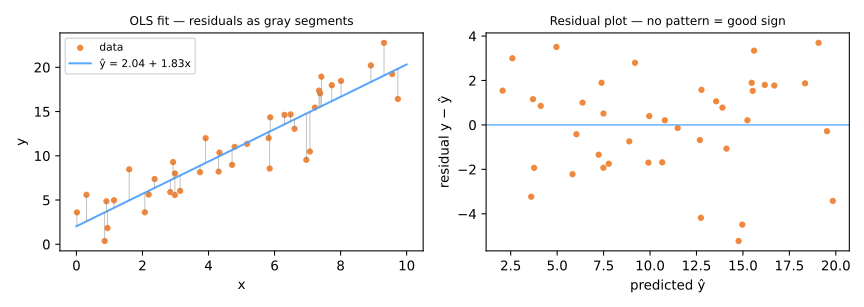
The residual plot puts \(e_i\) on the vertical axis against the fitted \(\hat{y}_i\) on the horizontal. A healthy one looks like nothing at all: a structureless band around zero. Any pattern is the model telling you which assumption it just broke.

Try to diagnose these four before reading the verdict — the top panel is what you would normally look at, and the point is that it is not enough:

Outlier and leverage are different things. An outlier has a large residual — the model missed it. A high-leverage point sits far from \(\bar{x}\) along the \(x\) axis, and it can drag the whole line toward itself. The dangerous case is a point with high leverage and a pull: it moves the line so effectively that its own residual ends up small, hiding the damage. That is the fourth case in the simulator. This is why "just drop the big residuals" is bad advice — the worst offenders do not have big residuals.

6. Measuring quality

Stage 5. Every metric below is a different way of summarizing the same vector of residuals \(e_i = y_i - \hat{y}_i\) into a single number. They disagree because they compress differently, so the names are worth reading in full before the formulas.

The acronyms are not arbitrary: each one spells out its own recipe, read right to left. RMSE is Error → Squared → Mean → Root: take each error, square it, average them, then take the square root. Read the name backwards and you have written the code.

Computing all four on the five points

The residuals from the worked example were \(-0.6,\ 0.6,\ 0.8,\ -1.0,\ 0.2\).

Read these back in context: the target values ranged from 2 to 6, so being off by roughly 0.7 on average is a meaningful error, not a rounding detail. MAE and RMSE are quotable to a non-technical audience — "the model misses by about 0.7" — while MSE is 0.48 squared units, which is not a sentence anyone can say out loud. That is the whole reason RMSE exists: it undoes the squaring so the number returns to the scale of the thing you are predicting.

MAE or RMSE?

They are not interchangeable, and the difference is exactly how they treat one big mistake. Two models on five predictions:

Identical MAE, and RMSE more than twice as large for B. MAE says the two models are equally good; RMSE says B is much worse, because it squares before averaging and the single error of 10 contributes 100 to the sum. Neither is right in the abstract — the question is what your problem costs. Delivery time being off by 10 minutes once is usually worse than being off by 2 minutes five times (use RMSE); for a demand forecast the total error may be what matters (use MAE). Choose before you look at the results, not after.

R², and why it is called that

R² compares your model against the laziest possible one. It is built from two sums: SSE, the sum of squared errors your line still makes, and SST, the total sum of squares, which is the error of ignoring \(x\) altogether.

SST, the total sum of squares, is the error you would make by ignoring \(x\) entirely and always predicting the mean \(\bar{y}\). SSE, the error sum of squares, is what your line still gets wrong. So R² answers: of the variation that was there to explain, what fraction did the model remove? Hence "coefficient of determination" — how much of \(y\) is determined by the features.

On the five points: \(R^2 = 1 - 2.40/8.80 = 0.727\), so the line removed about 73% of the original spread. And since \(r_{xy} = 0.853\) and \(0.853^2 = 0.727\), notice that in simple regression R² really is the squared correlation — that is where the symbol comes from. It stops being true the moment you add a second feature.

R² can be negative on test data, which surprises people who learned it as "a percentage". It means the model did worse than the flat line \(\hat{y}=\bar{y}\). Always fit that constant baseline (DummyRegressor) and report it: it is uncomfortable how often an elaborate model barely clears it.

7. Summary: a line in five lines

1. Regression to the mean is arithmetic, not a force: the slope is \(r_{xy}\,s_y/s_x\), and whenever the correlation is below 1 the predictions sit closer to the mean than the inputs.
2. A linear model is a weighted sum: each coefficient is the effect of its feature with the others fixed, and its size depends on the units, so it is not an importance.
3. \(X\) cannot be inverted; least squares takes the reachable point closest to \(y\): \(X^\top X w = X^\top y\). With one feature, \(\hat w_1 = \sum(x_i-\bar x)(y_i-\bar y)/\sum(x_i-\bar x)^2\) and \(\hat w_0 = \bar y - \hat w_1 \bar x\), so the line passes through \((\bar x, \bar y)\).
4. The residuals sum to zero and are orthogonal to every feature; their plot, not R², shows curves, funnels and dangerous points.
5. MAE, RMSE and R² summarize the same residuals: RMSE punishes big misses, R² compares with always predicting \(\bar y\), and all of them mean something only on data the model has not seen.

Fundamental lab — five points, from scratch

The problem. LinearRegression().fit hides the whole lesson in one call. This lab opens it: with only NumPy, it writes the model as a matrix product, tries the obvious inverse and watches it fail, solves the normal equations and checks, number by number, the hand calculation of section 4. The five points are those of the worked example, so every output can be checked on paper.

Step 1 — five points

Predict. Look at the five points before plotting them: \(x = 1, \dots, 5\) and \(y = 2, 4, 5, 4, 6\). Will the best line go up or down? Roughly how steep: closer to 0.5 or to 2 units of \(y\) per unit of \(x\)?

import numpy as np
import matplotlib.pyplot as plt
import time

np.set_printoptions(precision=4, suppress=True)
print("ready")

ready

x = np.array([1., 2., 3., 4., 5.])
y = np.array([2., 4., 5., 4., 6.])

plt.figure(figsize=(5,3.2))
plt.scatter(x, y, s=45, color='#f0883e', zorder=3)
plt.xlabel('x'); plt.ylabel('y'); plt.grid(alpha=.3)
plt.title('five observations'); plt.show()

print("x =", x)
print("y =", y)

x = [1. 2. 3. 4. 5.]
y = [2. 4. 5. 4. 6.]

Small numbers on purpose: everything that follows can be checked by hand. The cloud goes up, but not steadily: the fourth point (4, 4) is below the third (3, 5). No line passes through all five.

Step 2 — the matrix form

Predict. The model is \(\hat y_i = w_0 + w_1 x_i\). If every prediction is to be a row of one matrix product \(\hat y = Xw\), what must the first column of \(X\) hold, and what shape will \(X\) have?

X = np.column_stack([np.ones_like(x), x])
print("X =")
print(X)
print("\nshape of X:", X.shape, " ->", X.shape[0], "observations,", X.shape[1], "parameters")

X =
[[1. 1.]
 [1. 2.]
 [1. 3.]
 [1. 4.]
 [1. 5.]]

shape of X: (5, 2)  -> 5 observations, 2 parameters

The column of 1s is not a notational trick: multiplied by \(w_0\), it adds the intercept to every row, so the intercept is treated like any other weight. \(X\) is \(5 \times 2\): one row per observation, one column per parameter.

Step 3 — the obvious attempt: \(w = X^{-1}y\)

Predict. If \(\hat y = Xw\), the reflex is \(w = X^{-1}y\). Will NumPy compute it? If it refuses, is the problem only the shape of \(X\), or is there a deeper one?

try:
    w = np.linalg.inv(X) @ y
    print("w =", w)
except np.linalg.LinAlgError as err:
    print("LinAlgError:", err)

LinAlgError: Last 2 dimensions of the array must be square

rank_X   = np.linalg.matrix_rank(X)
rank_aug = np.linalg.matrix_rank(np.column_stack([X, y]))

print("rank(X)       =", rank_X)
print("rank([X | y]) =", rank_aug)
print()
if rank_aug > rank_X:
    print("y is NOT in the column space of X.")
    print("=> no w satisfies Xw = y exactly.")
else:
    print("y is in the column space: an exact solution exists.")

rank(X)       = 2
rank([X | y]) = 3

y is NOT in the column space of X.
=> no w satisfies Xw = y exactly.

Two obstacles, as in section 3. The first is the shape: inv only accepts square matrices, and \(X\) is \(5 \times 2\). The second is the one that matters: appending \(y\) raises the rank from 2 to 3, so \(y\) points in a direction the columns of \(X\) cannot reach. Five equations, two unknowns, no exact solution. With noisy data that is the normal situation, and it is why regression exists.

Simulation: your instinct, the special case. Section 3 claimed that \(w = X^{-1}y\) is not wrong, only a special case. Keep just the first two points, so that \(X\) becomes square, and compute \(w\) both ways: with np.linalg.inv and with the normal equations. Do they agree? What are the residuals, and why?

X2, y2 = X[:2], y[:2]                          # keep the first two points: X2 is 2 × 2
w_inv = np.linalg.inv(X2) @ y2                 # the reflex, now legal
w_ne  = np.linalg.solve(X2.T @ X2, X2.T @ y2)  # the normal equations
print("inv(X2) @ y2     =", w_inv)
print("normal equations =", w_ne)
print("residuals        =", y2 - X2 @ w_inv)

inv(X2) @ y2     = [0. 2.]
normal equations = [0. 2.]
residuals        = [0. 0.]

Step 4 — the normal equations

Predict. \(X^\top X\) will be \(2 \times 2\). Before running: which two numbers should \(w\) contain, if the hand calculation of section 4 is right? And what will \(\sum e_i\) and \(\sum e_i x_i\) be?

XtX = X.T @ X
Xty = X.T @ y

print("XᵀX =");  print(XtX);  print("shape:", XtX.shape, "-> square")
print("\nXᵀy =", Xty)

w = np.linalg.solve(XtX, Xty)     # solves the system; does NOT use inv()
print("\nw =", w)
print(f"fitted line:  ŷ = {w[0]:.1f} + {w[1]:.1f}·x")

XᵀX =
[[ 5. 15.]
 [15. 55.]]
shape: (2, 2) -> square

Xᵀy = [21. 71.]

w = [1.8 0.8]
fitted line:  ŷ = 1.8 + 0.8·x

yhat = X @ w
resid = y - yhat

print("ŷ =", yhat)
print("e =", resid)
print()
print("Σe      =", round(resid.sum(), 12) + 0.0)
print("Σe·x    =", round((resid * x).sum(), 12) + 0.0)
print("Xᵀe     =", (X.T @ resid).round(12) + 0.0)
print()
print("The two zeros above ARE the normal equations, written out:")
print("one per parameter. The residual is orthogonal to every column of X.")

ŷ = [2.6 3.4 4.2 5.  5.8]
e = [-0.6  0.6  0.8 -1.   0.2]

Σe      = 0.0
Σe·x    = 0.0
Xᵀe     = [0. 0.]

The two zeros above ARE the normal equations, written out:
one per parameter. The residual is orthogonal to every column of X.

plt.figure(figsize=(5,3.2))
plt.scatter(x, y, s=45, color='#f0883e', zorder=3, label='data')
xs = np.linspace(0.5, 5.5, 50)
plt.plot(xs, w[0] + w[1]*xs, color='#1F6B8E', lw=2, label=f'ŷ = {w[0]:.1f} + {w[1]:.1f}x')
for xi, yi, yh in zip(x, y, yhat):
    plt.plot([xi, xi], [yi, yh], color='#9E3B2E', lw=1.2, alpha=.8)
plt.legend(); plt.grid(alpha=.3); plt.xlabel('x'); plt.ylabel('y')
plt.title('the red segments are the residuals'); plt.show()

The matrix route lands on the hand result: \(\hat y = 1.8 + 0.8x\), the same predictions 2.6, 3.4, 4.2, 5.0 and 5.8 and the same residuals as the tables of section 4. The system is small enough to solve on paper too: \(5w_0 + 15w_1 = 21\) and \(15w_0 + 55w_1 = 71\); from the first, \(w_0 = (21 - 15w_1)/5\), and substituting in the second gives \(10w_1 = 8\), so \(w_1 = 0.8\) and \(w_0 = 1.8\). np.linalg.solve solves the system without ever forming an inverse. The two zeros are \(X^\top e = 0\): one equation per column of \(X\), the column of 1s giving \(\sum e_i = 0\) and the column of \(x\) giving \(\sum e_i x_i = 0\).

Simulation: the point that turns the line. Push one point 3 units down and refit, twice: first the middle point (\(x = 3\)), then the last one (\(x = 5\)). The push is the same; which one changes the slope more? And which of the two moved points ends up with the larger residual?

for i in [2, 4]:                               # the middle point (x = 3), then the last one (x = 5)
    y_moved = y.copy()
    y_moved[i] -= 3                            # the same push: 3 units down
    w_moved = np.linalg.solve(X.T @ X, X.T @ y_moved)
    e_moved = y_moved - X @ w_moved
    print(f"x = {x[i]:.0f} pushed down: w = {w_moved} · slope {w[1]:.1f} -> {w_moved[1]:.1f}"
          f" · residual of the moved point {e_moved[i]:+.1f}")

x = 3 pushed down: w = [1.2 0.8] · slope 0.8 -> 0.8 · residual of the moved point -1.6
x = 5 pushed down: w = [3.  0.2] · slope 0.8 -> 0.2 · residual of the moved point -1.0

To close the fundamental part. In one sentence each: (1) why is \(w = X^{-1}y\) not available for a dataset with more rows than columns? (2) What do the two zeros \(\sum e_i = 0\) and \(\sum e_i x_i = 0\) say about the residuals? (3) Why can a point with a small residual be the one that did most damage to the line?

Your turn (fundamental)

At home:

1. No intercept. Redo step 4 without the column of 1s (\(X\) with \(x\) only). Check that \(\sum e_i\) is no longer zero while \(\sum e_i x_i\) still is, and explain it with the phrase "one normal equation per parameter".
2. The three points of section 3. Run step 4 with \(x = 1, 2, 3\) and \(y = 2, 3, 7\). Do you get \(w_0 = -1\), \(w_1 = 2.5\) and \(\lVert e \rVert^2 = 1.5\)?
3. The four metrics. With mean_absolute_error, mean_squared_error and r2_score (from sklearn.metrics), compute MAE, MSE, RMSE and R² of yhat and check the 0.64, 0.48, 0.69 and 0.727 of section 6.

Advanced approach

The fundamental part fitted a line and judged it. This part looks underneath: what a coefficient can be trusted for, where the exact formula stops working, and the iterative route that replaces it, which the next lesson develops. The examples continue those of sections 1 to 7.

This part follows one path in four stages, drawn below: 1. trust the coefficients; 2. the limits of the closed form; 3. the gradient; 4. the landscape. Each stage links to its section, and in the slides a strip at the bottom shows which stage you are in.

Advanced approach slides

Click the slides and use the ← → arrows to navigate; F opens full screen and Esc shows every slide. Open the slides in a new tab

8. Assumptions behind the inferences

Stage 1. OLS predictions ask for very little. Interpreting coefficients, confidence intervals and p-values leans on the classical assumptions:

1. Linearity — the true relationship is approximately linear in the features;
2. Independence — residuals are uncorrelated with each other (beware time series);
3. Homoscedasticity — residual variance is constant across the range of \(\hat{y}\);
4. Normality of residuals — needed for exact intervals and p-values, not for the fit itself;
5. No severe multicollinearity — highly correlated features make individual coefficients unstable.

Each one has a picture in the residual plot of section 5: a curve breaks linearity, a funnel breaks homoscedasticity, waves over time break independence. The advanced lab meets the last one on real data: a year of stock-index closes whose residuals wander far from zero for weeks at a time.

Multicollinearity deserves a sentence of its own, because its symptom is counter-intuitive. With two features correlated at \(r = 0.99\), the data can barely tell their coefficients apart: \(X^\top X\) is nearly singular, so if the truth is \((w_1, w_2) = (1, 1)\), the pair \((2, 0)\) fits within about 2% of it and \((3, -1)\) within about 8%. Refit on a fresh sample and the individual estimates move by a whole unit or more — enough to flip a sign — while their sum stays pinned near 2, and the predictions with it. The model is fine; the interpretation of either coefficient alone is worthless.

9. When the closed form struggles

Stage 2. The formula \(\hat w = (X^\top X)^{-1}X^\top y\) solves the problem in one shot, but only while three things hold.

• Time. Solving the \(d \times d\) system costs \(O(d^3)\): doubling the number of features multiplies the time by about 8. A million features is hopeless.
• Memory. \(X^\top X\) has \(d^2\) numbers, however many rows there are: with 100,000 features (a text vectorized with TF-IDF passes that easily) it takes 80 GB before anything is solved. Step 5 of the lab measures both.
• Collinearity. When features are perfectly collinear, \(X^\top X\) is singular and there is no unique answer; when they are nearly collinear, the answer exists but is unstable, as in section 8.

And it has no equivalent at all for the models of the second half of this course — a neural network has no normal equations.

10. From the exact answer to the gradient

Stage 3. We have a formula that solves the problem in one shot, as long as it is available. So why does the rest of machine learning bother with iteration? Because what does generalize is the idea underneath.

Look again at how we got the closed form: we wrote down \(J(w)\), took its gradient, and asked where it vanishes. Gradient descent keeps the first two steps and gives up on the third. Instead of solving \(\nabla J = 0\) algebraically, it walks downhill until it gets there.

For simple regression, write the loss as a mean so the scale does not depend on \(n\):

Differentiate with respect to each parameter, using the chain rule and remembering \(e_i = y_i - w_0 - w_1x_i\):

Two things fall out of this, and both are worth pausing on.

First, set both to zero and you recover exactly the two identities the worked example satisfied: \(\sum e_i = 0\) and \(\sum e_i x_i = 0\). The closed form and the gradient are the same statement, approached from two directions.

Second, look at what the gradient is made of: it is a sum weighted by the residuals. Points the model already predicts well contribute \(e_i \approx 0\) and barely vote. Points it gets badly wrong dominate the step. The update rule

therefore reads, in plain language: move each parameter in the direction that the mistakes are pointing, by an amount proportional to how big the mistakes are. This is the sentence that will still be true, unchanged, when the model is a 100-layer network and \(\nabla J\) comes from backpropagation.

11. The landscape the gradient walks

Stage 4. The picture below makes the geometry concrete. On the left is \(J(w_0, w_1)\) as a landscape — every point is a candidate line, the color is its error, and the white cross is the closed-form optimum. Click to drop a starting guess and step downhill:

Now switch center x on and run it again from the same kind of starting point. Same data, same algorithm, dramatically different behavior.

Uncentered, the contours form a long narrow valley: \(w_0\) and \(w_1\) are strongly coupled, because moving the slope of a line whose \(x\) values are all far from zero also swings its height. The gradient points across the valley rather than along it, so the path zigzags and creeps. Centered, the valley becomes a bowl and the same steps go almost straight to the answer.

Choosing \(\eta\), doing this on batches rather than the whole dataset, and adding penalties to \(J\) that shrink the weights, are the subject of the next lesson: Gradient Descent & Regularization.

Advanced lab — where the closed form breaks, and a year of the Ibovespa

The fundamental lab solved the normal equations for five points. This part asks how far that formula goes: it measures what solving costs as the number of features grows, writes the iterative alternative, and then applies the very same two lines of algebra to real data, a year of daily closes of the Ibovespa, the main index of the São Paulo stock exchange (B3), to see what a well-fitted line can and cannot say about the future. Continue in the same notebook, in the same session: the steps below use x, y, X and w from steps 1 to 4.

Step 5 — where the closed form breaks: time and memory

Predict. Solving a \(d \times d\) system costs \(O(d^3)\). When \(d\) doubles, by how much should the time grow? And which runs out first on a laptop as \(d\) grows: patience or memory?

rng = np.random.default_rng(0)
print(f"{'d':>6} {'time':>10} {'ratio vs d/2':>14}")
previous = None
for d in [250, 500, 1000, 2000]:
    A = rng.standard_normal((d, d)); A = A @ A.T + d*np.eye(d)   # symmetric positive definite
    b = rng.standard_normal(d)
    t = min(( (lambda t0: (np.linalg.solve(A, b), time.perf_counter()-t0)[1])(time.perf_counter())
              for _ in range(3) ))
    ratio = f"{t/previous:.1f}×" if previous else "—"
    print(f"{d:>6} {t:>9.4f}s {ratio:>14}")
    previous = t

     d       time   ratio vs d/2
   250    0.0003s              —
   500    0.0014s           4.4×
  1000    0.0084s           5.9×
  2000    0.0793s           9.4×

print("memory needed just to STORE XᵀX (float64):\n")
for d in [1_000, 10_000, 50_000, 100_000]:
    gb = d*d*8 / 1e9
    verdict = "fits" if gb < 8 else "does NOT FIT in an ordinary laptop"
    print(f"  d = {d:>7}  ->  {gb:8.2f} GB   {verdict}")

print("\nA text vectorized with TF-IDF easily goes past 100 thousand columns.")
print("Then XᵀX is never even built — long before there is anything to invert.")

memory needed just to STORE XᵀX (float64):

  d =    1000  ->      0.01 GB   fits
  d =   10000  ->      0.80 GB   fits
  d =   50000  ->     20.00 GB   does NOT FIT in an ordinary laptop
  d =  100000  ->     80.00 GB   does NOT FIT in an ordinary laptop

A text vectorized with TF-IDF easily goes past 100 thousand columns.
Then XᵀX is never even built — long before there is anything to invert.

The timings are those of one run and depend on the machine; what matters is the ratio column. At small sizes the fixed cost of calling the routine and the parallelism of the linear-algebra library weigh more than the arithmetic, so the ratio starts well below 8 and climbs toward it as \(d\) grows (9.4 here, at \(d = 2000\)). Time is bad but manageable. Memory is what stops you: \(X^\top X\) needs \(8d^2\) bytes whatever the number of rows, 80 GB at 100,000 features. That is section 9, measured.

Simulation: gradient descent, written by hand. Section 10 derived the two derivatives. Write the descent for the five points: start at \(w_0 = w_1 = 0\), update both weights with \(w \leftarrow w - \eta\,\nabla J\) for 2000 iterations, and try \(\eta = 0.01, 0.05, 0.08\) and \(0.09\). Which rates land on the closed form of step 4, \((1.8, 0.8)\)? What happens to the last one?

def descend(x, y, eta, iters=2000):
    w0 = w1 = 0.0
    n = len(x)
    for _ in range(iters):
        e = y - (w0 + w1 * x)                  # residuals of the current line
        w0 -= eta * (-2 / n * e.sum())         # ∂J/∂w0 = −(2/n)·Σe
        w1 -= eta * (-2 / n * (e * x).sum())   # ∂J/∂w1 = −(2/n)·Σe·x
    return w0, w1

for eta in [0.01, 0.05, 0.08, 0.09]:
    w0, w1 = descend(x, y, eta)
    print(f"eta {eta:.2f}: w0 = {w0:.4g} · w1 = {w1:.4g}")

eta 0.01: w0 = 1.798 · w1 = 0.8005
eta 0.05: w0 = 1.8 · w1 = 0.8
eta 0.08: w0 = 1.8 · w1 = 0.8
eta 0.09: w0 = -2.245e+105 · w1 = -8.104e+105

Step 6 — a year of the Ibovespa

Predict. The model will be the simplest possible: \(y\) = the day's close, \(x\) = the position of the trading day in the window (1, 2, 3, …). Over a year, roughly how many trading days do you expect? And how far apart will the scales of the two columns of \(X\) be?

# yfinance does not come with Colab by default
%pip install -q yfinance

import yfinance as yf
import pandas as pd

print("yfinance", yf.__version__)

yfinance 1.7.0

raw = yf.download("^BVSP", period="1y", progress=False, auto_adjust=True)

close = raw["Close"]
if isinstance(close, pd.DataFrame):     # recent versions return two-level columns
    close = close.iloc[:, 0]
close = close.dropna()

print(f"{len(close)} trading days, from {close.index[0]:%m/%d/%Y} to {close.index[-1]:%m/%d/%Y}")
print(f"first close:            {close.iloc[0]:>12,.0f}")
print(f"last close:             {close.iloc[-1]:>12,.0f}")
print(f"change over the window: {100*(close.iloc[-1]/close.iloc[0]-1):>11.1f}%")

249 trading days, from 10/23/2025 to 10/23/2026
first close:                 145,721
last close:                  205,083
change over the window:        40.7%

y_ibov = close.to_numpy(dtype=float)
x_ibov = np.arange(1, len(y_ibov) + 1, dtype=float)

print("x:", x_ibov[:6], "...", x_ibov[-3:])
print("y:", np.round(y_ibov[:6]), "...", np.round(y_ibov[-3:]))
print("\nn =", len(y_ibov))

x: [1. 2. 3. 4. 5. 6.] ... [247. 248. 249.]
y: [145721. 146172. 146969. 147429. 148633. 148780.] ... [206495. 204120. 205083.]

n = 249

yfinance reads the public Yahoo Finance data; ^BVSP is the index's code. A year has about 250 trading days (249 in this window): weekends and holidays have no price, so they are not observations, and \(x\) counts trading days, not calendar days. Look at the scales: \(y\) is in the hundreds of thousands, \(x\) runs from 1 to 249, and the column of 1s is 1. Keep that in mind: it is the subject of the next simulation.

Simulation: what centering does to the descent. The \(x\) of the Ibovespa runs from 1 to 249, far from zero; section 11 said this makes gradient descent zigzag. Measure it where it is quick, on the five points: count how many iterations the descent of the previous simulation needs to get both weights within 0.001 of the exact solution, with the raw \(x\) and with the centered \(x - \bar x\), for \(\eta = 0.01, 0.05, 0.08, 0.3\) and \(0.45\).

def steps_to_answer(x, y, eta, tol=1e-3):
    """iterations until both weights are within tol of the exact solution"""
    A = np.column_stack([np.ones_like(x), x])
    target = np.linalg.solve(A.T @ A, A.T @ y)
    w0 = w1 = 0.0
    n = len(x)
    for k in range(1, 10_001):
        e = y - (w0 + w1 * x)
        w0, w1 = w0 + eta * 2 / n * e.sum(), w1 + eta * 2 / n * (e * x).sum()
        if not np.isfinite(w1) or abs(w1) > 1e6:
            return 'diverges'
        if abs(w0 - target[0]) < tol and abs(w1 - target[1]) < tol:
            return k
    return '> 10000'

xc = x - x.mean()
print(f"{'eta':>5} {'raw x':>9} {'centered x':>11}")
for eta in [0.01, 0.05, 0.08, 0.3, 0.45]:
    print(f"{eta:5.2f} {steps_to_answer(x, y, eta):>9} {steps_to_answer(xc, y, eta):>11}")

  eta     raw x  centered x
 0.01      2153         413
 0.05       428          80
 0.08       266          48
 0.30  diverges          10
 0.45  diverges          30

Step 7 — the same two lines of algebra

Predict. The code that fitted five invented points will now fit 249 real closes, without changing a line. Over this window the index rose 40.7%. Will the fitted line rise steeply? Will it pass close to today's close?

X_ibov = np.column_stack([np.ones_like(x_ibov), x_ibov])

# exactly the same two lines as in step 4
w_ibov = np.linalg.solve(X_ibov.T @ X_ibov, X_ibov.T @ y_ibov)

print("X_ibov.shape =", X_ibov.shape)
print("w =", w_ibov)
print(f"\nline:  close ≈ {w_ibov[0]:,.0f}  +  {w_ibov[1]:,.1f} · day")
print(f"\nthat is: the line credits {w_ibov[1]:,.1f} points of gain to each trading day.")

X_ibov.shape = (249, 2)
w = [161854.1202    116.1611]

line:  close ≈ 161,854  +  116.2 · day

that is: the line credits 116.2 points of gain to each trading day.

yhat_ibov = X_ibov @ w_ibov
res_ibov  = y_ibov - yhat_ibov

plt.figure(figsize=(9, 4))
plt.plot(x_ibov, y_ibov, color='#f0883e', lw=1.2, label='Ibovespa close')
plt.plot(x_ibov, yhat_ibov, color='#1F6B8E', lw=2,
         label=f'line: {w_ibov[0]:,.0f} + {w_ibov[1]:,.1f}·day')
plt.xlabel('day (position in the window)'); plt.ylabel('points')
plt.title('a year of Ibovespa and the least-squares line')
plt.legend(); plt.grid(alpha=.3); plt.show()

plt.figure(figsize=(9, 2.4))
plt.axhline(0, color='#1F6B8E', lw=1.5)
plt.plot(x_ibov, res_ibov, color='#9E3B2E', lw=1)
plt.xlabel('day'); plt.ylabel('residual'); plt.title('the residuals, alone')
plt.grid(alpha=.3); plt.show()

The code does not know it is looking at a stock index: \(X\) is now \(249 \times 2\) instead of \(5 \times 2\), and nothing else changed. The line gains 116.2 points per trading day, about 29,000 over the window, well short of the 59,000 the index actually gained (from 145,721 to 205,083). The slope is not "last close minus first close": least squares balances every day of the year, and this window had a climb in the first months, a long dip in the middle and a sharp rise in the last two months. On this window the line's value on the last day is 161,854 + 116.2 × 249 ≈ 190,800, some 14,000 points below the actual close. Look at the residual plot before moving on: the residuals do not scatter around zero like dust; they wander, staying above zero for weeks and then below.

Step 8 — how much the line explains

Predict. Section 8 listed independence of the residuals among the assumptions. In the residual plot of step 7, today's residual looks a lot like yesterday's. Will the correlation between neighboring residuals be near 0, near 0.5 or near 1?

n_ibov = len(y_ibov)
sse = res_ibov @ res_ibov
sst = ((y_ibov - y_ibov.mean())**2).sum()
r2  = 1 - sse/sst
s   = np.sqrt(sse/(n_ibov - 2))
rho = np.corrcoef(res_ibov[:-1], res_ibov[1:])[0, 1]

print(f"R²                                   = {r2:.4f}")
print(f"typical size of the residual (s)     = {s:,.0f} points")
print(f"   ... as % of today's index         = {100*s/y_ibov[-1]:.1f}%")
print(f"correlation of neighboring residuals = {rho:.4f}")

R²                                   = 0.3674
typical size of the residual (s)     = 11,001 points
   ... as % of today's index         = 5.4%
correlation of neighboring residuals = 0.9797

Three numbers. R² is the share of the spread around the mean that the line removed: 37% in this window. \(s\) is the typical residual, 11,001 points, 5.4% of the index; it divides by \(n - 2\) instead of \(n\) because two parameters were estimated from the data. The third is the one that matters: the correlation between today's residual and yesterday's is 0.98. The independence assumption is plainly broken. A price does not oscillate around a trend: each day starts from where the previous one ended. Every error bar the classical theory offers assumes the opposite.

Step 9 — where does the index close the year?

Predict. Extending the line to December 31 gives one number. The notebook also computes a 95% interval for it. Will the interval be narrow enough to tell whether the index goes up or down by year end?

last = close.index[-1]
year_end = pd.Timestamp(last.year, 12, 31)

# business days left (B3 holidays are not removed, so it comes out a little high)
days_left = len(pd.bdate_range(last + pd.Timedelta(days=1), year_end))
day_end = n_ibov + days_left

forecast = w_ibov[0] + w_ibov[1]*day_end

# standard error of PREDICTION: grows as x0 moves away from the center of the data
Sxx = ((x_ibov - x_ibov.mean())**2).sum()
se_pred = s*np.sqrt(1 + 1/n_ibov + (day_end - x_ibov.mean())**2/Sxx)
lo, hi = forecast - 1.96*se_pred, forecast + 1.96*se_pred

print(f"last trading day in the window: {last:%m/%d/%Y}  (day {n_ibov})")
print(f"trading days to 12/31:          {days_left}  ->  day {day_end:.0f}\n")
print(f"FORECAST FOR YEAR END:  {forecast:,.0f} points")
print(f"today:                  {y_ibov[-1]:,.0f} points")
print(f"implies:                {100*(forecast/y_ibov[-1]-1):+.1f}%\n")
print(f"95% interval: [{lo:,.0f} ; {hi:,.0f}]   (width: {hi-lo:,.0f} points)")
print(f"does the interval contain today's value? {'YES' if lo <= y_ibov[-1] <= hi else 'no'}")

last trading day in the window: 10/23/2026  (day 249)
trading days to 12/31:          49  ->  day 298

FORECAST FOR YEAR END:  196,470 points
today:                  205,083 points
implies:                -4.2%

95% interval: [174,616 ; 218,325]   (width: 43,709 points)
does the interval contain today's value? YES

xs = np.linspace(1, day_end, 400)
se_xs = s*np.sqrt(1 + 1/n_ibov + (xs - x_ibov.mean())**2/Sxx)
line_xs = w_ibov[0] + w_ibov[1]*xs

plt.figure(figsize=(9, 4.4))
plt.fill_between(xs, line_xs - 1.96*se_xs, line_xs + 1.96*se_xs,
                 color='#1F6B8E', alpha=.12, label='95% interval')
plt.plot(x_ibov, y_ibov, color='#f0883e', lw=1.2, label='observed close')
plt.plot(xs, line_xs, color='#1F6B8E', lw=2, label='extrapolated line')
plt.axvline(n_ibov, color='#9E3B2E', ls='--', lw=1.2)
plt.scatter([day_end], [forecast], color='#9E3B2E', s=70, zorder=5,
            label=f'12/31: {forecast:,.0f}')
plt.xlabel('day (position in the window)'); plt.ylabel('points')
plt.title('the climax: the line carried to year end')
plt.legend(loc='upper left', fontsize=9); plt.grid(alpha=.3); plt.show()

The interval is not "the line ± \(s\)". Predicting one new observation at \(x_0\) adds three uncertainties: that of the new point itself (the 1 under the root), that of the line's height (\(1/n\)) and that of its slope, which grows with the distance from the center of the data, \((x_0 - \bar x)^2/\sum(x_i - \bar x)^2\): the price of extrapolating. Forty-nine trading days past a window of 249, that price is still small; almost all the width comes from \(s\) itself. On this run the line points to 196,470 on December 31, 4.2% below an index that rose 40.7% in the year, and the interval, 43,709 points wide, contains today's value. In the model's own terms, it does not know whether the index will end the year up or down. And the interval is optimistic: it assumes independent errors, the assumption step 8 showed broken.

Step 10 — the honest test

Predict. Fit the line on one year and use it to predict the last day of the next year, then compare with what happened. Do you expect an error near \(s\), the 11,000 points of step 8, or much larger?

d2 = yf.download("^BVSP", period="2y", progress=False, auto_adjust=True)["Close"]
if isinstance(d2, pd.DataFrame):
    d2 = d2.iloc[:, 0]
d2 = d2.dropna()

v  = d2.to_numpy(dtype=float)
n2 = len(v)
cut = n2 // 2                        # train on the first half (~1 year)

x_tr = np.arange(1, cut + 1, dtype=float)
y_tr = v[:cut]
X_tr = np.column_stack([np.ones_like(x_tr), x_tr])
w_tr = np.linalg.solve(X_tr.T @ X_tr, X_tr.T @ y_tr)

predicted = w_tr[0] + w_tr[1]*n2     # one year past the end of training
actual    = v[-1]

print(f"train:  {d2.index[0]:%m/%d/%Y} to {d2.index[cut-1]:%m/%d/%Y}  ({cut} trading days)")
print(f"target: {d2.index[-1]:%m/%d/%Y}  (day {n2})\n")
print(f"the line predicted: {predicted:>12,.0f}")
print(f"what happened:      {actual:>12,.0f}")
print(f"error:              {predicted-actual:>+12,.0f} points   ({100*(predicted/actual-1):+.1f}%)")

train:  10/23/2024 to 10/22/2025  (249 trading days)
target: 10/23/2026  (day 498)

the line predicted:      164,118
what happened:           205,083
error:                   -40,965 points   (-20.0%)

This is the test that counts, the one the validation lesson builds on: apply the procedure to the past and compare with what happened, on data it has not seen. Fitted on the year up to October 2025, the line predicted 164,118 for October 2026; the index closed at 205,083. The error, 40,965 points or 20%, is almost four times the \(s\) of step 8. The algebra is flawless: the normal equations returned the best line for that window. What fails is the question. R² measures the fit to the past, not the ability to predict; extrapolating repeats an assumption, that the trend goes on, which no data confirmed; and with residuals that wander (correlation 0.98), the slope you measured is largely the path that happened to occur. The line is good for describing the window: on average, so many points per trading day. It does not answer the question everyone wants to ask.

To close the lesson. In one sentence each: (1) what runs out first when the number of features grows, and what replaces the closed form then? (2) Why does centering \(x\) speed up gradient descent without changing the line it finds? (3) Why is an R² computed on the past no evidence that the line can predict the future?

Your turn (advanced)

At home, with more time:

1. The cost, measured further. Extend step 5 to d = 4000. Does the ratio stay near 8? Where does it start to move away, and why?
2. The window changes the trend. Redo steps 6 and 7 with period="5y" and with period="6mo", and note the slope each time. If "the trend of the Ibovespa" were a fact of the world, should it depend this much on the window you chose?
3. A logarithm instead of the level. Fit the line to \(\log(\text{close})\): the slope becomes roughly the growth rate per trading day and the forecast is \(e^{\hat y}\). Why is a straight line in the logarithm more defensible for a price than a straight line in the level? (Hint: what does a line in the level assume about gaining 100 points from 50,000 or from 200,000?)

Class materials

References

• Legendre, A.-M. "Nouvelles méthodes pour la détermination des orbites des comètes." Courcier (1805) — appendix Sur la Méthode des moindres quarrés. full text
• Gauss, C. F. "Theoria motus corporum coelestium in sectionibus conicis solem ambientium." Perthes & Besser (1809). full text
• Galton, F. "Regression toward Mediocrity in Hereditary Stature." J. Anthropological Institute 15 (1886). full text
• Hanley, J. A. ""Transmuting" Women into Men: Galton's Family Data on Human Stature." The American Statistician 58 (2004). DOI
• Anscombe, F. J. "Graphs in Statistical Analysis." The American Statistician 27 (1973). DOI
• Cook, R. D. "Detection of Influential Observation in Linear Regression." Technometrics 19 (1977). DOI

Quiz

The quiz covers the fundamental approach.