The oldest algorithm in the course
Legendre
publishes least squares to fit comet orbits
Gauss
claims he had used it since then
Galton
studies human height, and the word regression appears
The path of this lesson
- Galton's puzzleregression to the mean; the slope is the correlation
- The modelŷ = Xw; why not invert X; reading the coefficients
- Least squaresminimize the squared residuals; the exact solution
- Residuals & qualityresidual plots, error metrics, R², assumptions
- Toward the gradienta sum weighted by the residuals
Galton's puzzle
- Heights of 928 adult children and their parents.
- He was looking for the strength of heredity.
The children come back toward the mean
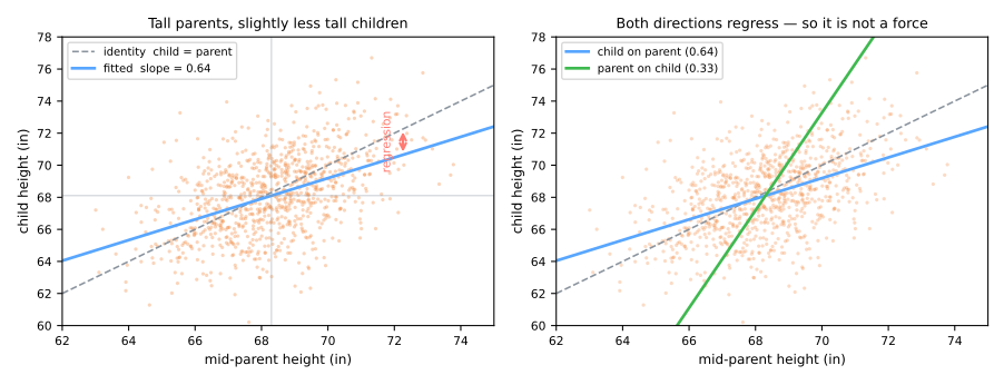
Dashed line: identity (the child equals the parent). The fitted line is flatter: 3 inches above the mean in the parents → only about 2 in the child.
The slope is the correlation, with units
\[ \hat{w}_1 = r_{xy}\,\frac{s_y}{s_x} = 0.46 \times \frac{2.52}{1.80} \approx 0.64 \]correlation \(r\)
no units; how tightly the points follow a line
slope \(\hat w_1\)
units of \(y\) per unit of \(x\); the same as \(r\) only when \(s_x = s_y\)
Simulator: regression to the mean
Both variables have the same spread here, so the slope is the correlation. Lower the correlation and watch the line flatten.
Regression to the mean is not a force
- Regress parent on child: that line is flatter too. Children cannot pull their parents toward the mean.
- It is arithmetic: a measurement is signal + noise. An extreme value had help from luck; the signal comes back, the luck does not.
tutoring
the worst students improve — they would have anyway
the magazine jinx
an exceptional season is followed by a normal one
the clinic
part of the drop in pressure is regression; only a control group separates it
The model
\[ \hat{y} = w_0 + w_1 x_1 + w_2 x_2 + \dots + w_d x_d \qquad\text{or}\qquad \hat y = Xw \]- \(w_j\): change in \(\hat{y}\) per unit of \(x_j\), holding the other features fixed.
- \(w_0\): the prediction when every feature is zero (a column of 1s in \(X\)).
Why not just invert \(X\)?
- \(X\) is not square (\(3 \times 2\)): it has no inverse.
- There is no exact solution anyway: 3 equations, 2 unknowns.
What we do instead: the closest reachable point
Minimize \(\lVert y - Xw\rVert^2\). Setting the gradient to zero gives the normal equations:
\[ X^\top X\,w = X^\top y \quad\Rightarrow\quad \begin{cases} 3w_0 + 6w_1 = 12 \\ 6w_0 + 14w_1 = 29 \end{cases} \quad\Rightarrow\quad w_0 = -1,\; w_1 = 2.5 \]fitted
1.5, 4, 6.5
residuals
0.5, −1, 0.5
\(\lVert e\rVert^2\)
\(X^\top X\) is \(2\times 2\): square. We never invert \(X\).
Your instinct is the special case
Keep only two points: two equations, two unknowns.
\[ X = \begin{pmatrix} 1 & 1 \\ 1 & 2 \end{pmatrix}, \quad X^{-1} = \begin{pmatrix} 2 & -1 \\ -1 & 1 \end{pmatrix}, \quad w = X^{-1}y = \begin{pmatrix} 1 \\ 1 \end{pmatrix} \]Least squares gives the same answer: \((X^\top X)^{-1}X^\top = X^{-1}\).
Reading the coefficients
\[ \widehat{\text{price}} = 50000 + 3200\cdot\text{area} - 1500\cdot\text{age} \]3200: among apartments of the same age, one extra m² goes with R$ 3200 more.- It is not "bigger apartments cost 3200 more per m²": if newer buildings are larger, the raw relation mixes both effects.
Least squares: which line?
\[ J(w) = \sum_{i=1}^{n} (y_i - \hat{y}_i)^2 = \lVert y - Xw \rVert^2 \]why vertical?
the job is to predict \(y\): an error is measured along \(y\). Perpendicular distances are PCA, another question.
why squared?
- smooth: there is a closed form
- one big error costs more than several small
- Gaussian noise → maximum likelihood
Simulator: drag the points
Predict. Drag one point far from the rest. Does the line move a little or a lot?
The exact solution, for one feature
\[ \hat{w}_1 = \frac{\sum_i (x_i - \bar{x})(y_i - \bar{y})}{\sum_i (x_i - \bar{x})^2} = r_{xy}\frac{s_y}{s_x}, \qquad \hat{w}_0 = \bar{y} - \hat{w}_1 \bar{x} \]Worked by hand: five points
| \(x\) | \(y\) | \(x-\bar x\) | \(y-\bar y\) | product | \((x-\bar x)^2\) |
|---|---|---|---|---|---|
| 1 | 2 | −2 | −2.2 | 4.4 | 4 |
| 2 | 4 | −1 | −0.2 | 0.2 | 1 |
| 3 | 5 | 0 | 0.8 | 0.0 | 0 |
| 4 | 4 | 1 | −0.2 | −0.2 | 1 |
| 5 | 6 | 2 | 1.8 | 3.6 | 4 |
| 8.0 | 10 |
\(\bar x = 3,\ \bar y = 4.2\)
\[ \hat w_1 = \tfrac{8.0}{10} = 0.8 \] \[ \hat w_0 = 4.2 - 0.8 \times 3 = 1.8 \]The residuals always balance
| \(x\) | \(y\) | \(\hat y\) | \(e = y - \hat y\) |
|---|---|---|---|
| 1 | 2 | 2.6 | −0.6 |
| 2 | 4 | 3.4 | 0.6 |
| 3 | 5 | 4.2 | 0.8 |
| 4 | 4 | 5.0 | −1.0 |
| 5 | 6 | 5.8 | 0.2 |
\(\sum e_i = 0\) and \(\sum e_i x_i = -0.6+1.2+2.4-4.0+1.0 = 0\). True for every OLS fit with an intercept.
In scikit-learn
from sklearn.linear_model import LinearRegression

model = LinearRegression().fit(X_train, y_train)
model.coef_, model.intercept_
y_pred = model.predict(X_test)
Residuals: what the model failed to explain
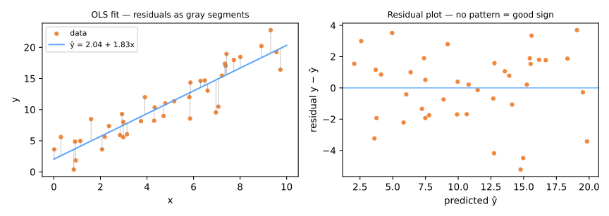
The residual plot: \(e_i\) against \(\hat y_i\).
A healthy one looks like nothing at all: a band around zero.
Any pattern says which assumption broke.
Simulator: diagnose before reading the verdict
Predict. For each dataset, look only at the residual plot and decide: fine, curve, funnel or a dangerous point?
Reading a residual plot
| what you see | what it means | what to do |
|---|---|---|
| structureless band | the linear form fits | nothing |
| U or ∩ curve | a nonlinear relationship | polynomial terms, or transform \(x\) |
| funnel | heteroscedasticity: noise grows with \(\hat y\) | transform \(y\) (often log) |
| isolated extreme point | outlier or high leverage | investigate it; never delete it silently |
| waves over the index | correlated errors (time) | a time-series model |
Measuring quality: four ways to summarize the residuals
| metric | formula | units |
|---|---|---|
| MAE | \(\frac{1}{n}\sum \lvert e_i \rvert\) | of \(y\) |
| MSE | \(\frac{1}{n}\sum e_i^2\) | \(y\) squared |
| RMSE | \(\sqrt{\text{MSE}}\) | of \(y\) |
| R² | \(1 - \frac{\sum e_i^2}{\sum (y_i - \bar{y})^2}\) | none |
The name is the recipe, read right to left:
RMSE = Error → Squared → Mean → Root.
Mean Absolute Error, Mean Squared Error, Root Mean Squared Error, coefficient of determination.
On the five points
Residuals: −0.6, 0.6, 0.8, −1.0, 0.2
MAE
MSE
RMSE
MAE or RMSE?
| errors | MAE | RMSE | |
|---|---|---|---|
| Model A | 2, 2, 2, 2, 2 | 2.0 | 2.0 |
| Model B | 0, 0, 0, 0, 10 | 2.0 | 4.47 |
RMSE squares before averaging: the single 10 contributes 100. Neither metric is right in the abstract: choose the one your problem's costs call for, before looking at the results.
R²: against the laziest model
\[ R^2 = 1 - \frac{\text{SSE}}{\text{SST}}, \qquad \text{SSE} = \sum (y_i - \hat y_i)^2, \quad \text{SST} = \sum (y_i - \bar y)^2 \]- SST: the error of always predicting \(\bar y\). SSE: what the line still gets wrong.
- Five points: \(R^2 = 1 - 2.40/8.80 = 0.727\), and \(r = 0.853\), \(0.853^2 = 0.727\).
DummyRegressor), and evaluate on held-out data.Assumptions behind the inferences
- Linearity
- Independence of residuals
- Homoscedasticity: constant spread
- Normality: for intervals and p-values, not for the fit
- No severe multicollinearity
two features with \(r = 0.99\)
Truth \((1, 1)\); \((2, 0)\) fits within 2%, \((3, -1)\) within 8%.
A new sample can flip a sign, while the sum stays near 2.
The predictions are fine; one coefficient alone means nothing.
From the exact answer to the gradient
The closed form stops being available: \(O(d^3)\), collinear columns, and models (neural networks) that have no normal equations.
\[ \frac{\partial J}{\partial w_0} = -\frac{2}{n}\sum_i e_i, \qquad \frac{\partial J}{\partial w_1} = -\frac{2}{n}\sum_i e_i x_i, \qquad w \leftarrow w - \eta\,\nabla J(w) \]Simulator: walking down the loss surface
Predict. Run it, then switch center x on and run it again from the same kind of start. What changes in the path?
Why scaling comes before fitting
uncentered \(x\)
A long narrow valley. Changing the slope of a line whose \(x\) values are all far from zero also swings its height, so \(w_0\) and \(w_1\) are coupled. The gradient points across the valley: the path zigzags and creeps.
centered \(x\)
A round bowl. The gradient points at the bottom, and the same steps go almost straight to the answer.
Schematic: contour lines of \(J(w_0, w_1)\), the optimum (green) and the steps of gradient descent (orange).
Summary
- Regression to the mean is arithmetic, not a force.
- Least squares = the reachable point closest to \(y\): \(X^\top X w = X^\top y\).
- The residuals are orthogonal to the features; plot them.
- MAE, RMSE, R²: different summaries of the same residuals; R² against \(\bar y\).
- The gradient is a sum weighted by the residuals.