Logistic Regression
This lesson opens the classification block of the course. Until now the target was a number (a price, a grade); from here on it is a category: survived or not, spam or not, which of three species. The first model is logistic regression (Cox, 1958; its curve goes back to Verhulst, 1838). Despite the name, it is a classifier: the default first model for any classification problem, a fixture of credit scoring and medicine, and the gateway to neural networks, where a single neuron is a logistic regression.
You already own every piece it is built from: the linear score of linear regression and the gradient descent loop. What is new is one function (the sigmoid), one loss (cross-entropy) and one way of reading coefficients (odds). Every number below comes from running the code on this page, and every figure from a short script next to it.
The lesson follows one pipeline in five stages, drawn below: 1. why not a line, what goes wrong when linear regression classifies; 2. score → probability, the sigmoid, the decision boundary and the odds; 3. loss and training, cross-entropy and gradient descent; 4. beyond the line, curved boundaries and more than two classes; 5. probability → label, the threshold and when to use the model. Each stage links to its section, and in the slides a strip at the bottom shows which stage you are in.
- Why not a linea straight line fails at classifying
- Score → probabilitysigmoid, decision boundary, odds
- Loss & trainingcross-entropy, not squared error; gradient descent
- Beyond the linecurved boundaries; many classes with softmax
- Probability → labelthe threshold is a choice; when to use the model
Slides
Click the slides and use the ← → arrows to navigate; F goes full screen and Esc shows every slide. Open the slides in a new tab
What classification is
A classification problem has a target \(y\) that takes values in a finite set of classes:
| classes | examples | |
|---|---|---|
| binary | 2, coded 0 and 1 | pass/fail, fraud/legit, malignant/benign, survived/died |
| multiclass | \(k > 2\) | iris species, digit 0–9, product category |
Almost every classifier works in two steps. First it computes, for each example, a score or a probability for each class ("this passenger survives with probability 0.94"). Then a threshold turns that number into a label ("0.94 ≥ 0.5, so: survived"). Keep the two stages apart in your head: most of this lesson is about the first, and the last section is about the second. The simplest way to grade the labels is accuracy, the fraction predicted correctly. It is enough for this lesson; its traps and the better metrics are the subject of Classification Metrics.
Why not a straight line?
Stage 1. The obvious first attempt: code the classes as 0 and 1 and fit a linear regression, then call "pass" anything the line puts above 0.5. Take 23 students, the hours they studied, and whether they passed. Then add five students who studied a lot, and passed, as you would expect. (One detail of the code: scikit-learn's LogisticRegression adds by default the L2 penalty you met in Ridge; C=np.inf switches it off, so we fit exactly the model of this lesson. The penalty, and how to tune C, come back in the cross-validation lesson.)
import numpy as np
from sklearn.linear_model import LinearRegression, LogisticRegression

hours = np.arange(1, 12.5, 0.5)                    # 23 students: 1, 1.5, ..., 12 hours of study
passed = np.array([0] * 11 + [1, 0] + [1] * 10)    # fail up to 6 h, a mixed zone, pass from 7.5 h
far = np.array([25, 30, 35, 40, 45])               # five students who studied a lot, and passed

for label, h, y in [('23 students', hours, passed),
                    ('+ 5 far passers', np.r_[hours, far], np.r_[passed, [1] * 5])]:
    X = h.reshape(-1, 1)
    line = LinearRegression().fit(X, y)
    logit = LogisticRegression(C=np.inf).fit(X, y)     # C=np.inf: the plain model, no penalty
    out = line.predict(X)
    print(f"{label}:")
    print(f"  line     outputs from {out.min():.2f} to {out.max():.2f}, crosses 0.5 at "
          f"{(0.5 - line.intercept_) / line.coef_[0]:.2f} h, errors: {((out >= 0.5) != y).sum()}")
    print(f"  logistic crosses 0.5 at {-logit.intercept_[0] / logit.coef_[0, 0]:.2f} h, "
          f"errors: {(logit.predict(X) != y).sum()}")
23 students:
  line     outputs from -0.23 to 1.18, crosses 0.5 at 6.67 h, errors: 2
  logistic crosses 0.5 at 6.75 h, errors: 2
+ 5 far passers:
  line     outputs from 0.31 to 1.39, crosses 0.5 at 8.66 h, errors: 4
  logistic crosses 0.5 at 6.75 h, errors: 2
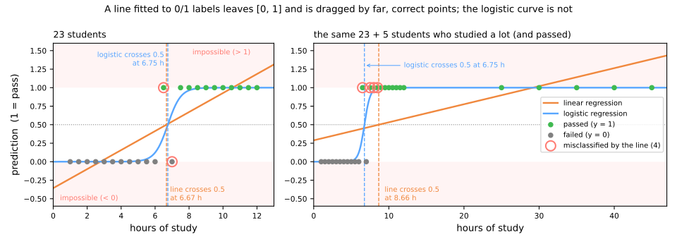
Two problems, both visible in the figure:
- The line leaves [0, 1]. It predicts −0.23 for the student who studied one hour and 1.18 for the one who studied twelve. Neither is a probability, so "how sure is the model?" has no answer.
- Correct points hurt it. The five far students are easy cases, labeled exactly as anyone would guess. But least squares wants the line to pass near them, which flattens its slope and drags the 0.5 crossing from 6.67 h to 8.66 h. Three students who studied 7.5 to 8.5 hours and passed are now called "fail" (the one who failed with 7 hours becomes right by accident), and the errors go from 2 to 4, caused by data that agreed with the model.
The logistic curve crosses 0.5 at 6.75 hours in both cases and makes the same 2 errors (the student who passed with 6.5 hours and the one who failed with 7, which no threshold on hours can get right). A student with 45 hours sits on the flat part of the curve at probability ≈ 1, where there is nothing left to correct, so it barely pulls on the fit. That flat part is the whole idea.
From line to probability
Stage 2. Logistic regression keeps the linear score you know,
and passes it through the sigmoid (or logistic) function, which squashes any real number into the interval (0, 1):
Three values are worth memorizing: \(\sigma(0) = 0.5\); large positive \(z\) gives \(\hat p \to 1\); large negative \(z\) gives \(\hat p \to 0\). The prediction is class 1 when \(\hat p \geq 0.5\), which is the same as \(z \geq 0\).
By hand, then with scikit-learn
Fitted on the 23 students, the model is \(w = 2.619\) per hour and \(b = -17.681\). Three new students:
| hours \(x\) | \(z = 2.619x - 17.681\) | \(e^{-z}\) | \(\hat p = 1/(1+e^{-z})\) | class |
|---|---|---|---|---|
| 4 | −7.205 | 1346 | 0.001 | 0 (fail) |
| 6 | −1.967 | 7.149 | 0.123 | 0 (fail) |
| 7.5 | 1.962 | 0.1406 | 0.877 | 1 (pass) |
A calculator is enough. Now the same with the library. decision_function returns the score \(z\), predict_proba the probabilities of each class (column 1 is class 1), predict the label:
def sigmoid(z):
    return 1 / (1 + np.exp(-z))

model = LogisticRegression(C=np.inf).fit(hours.reshape(-1, 1), passed)
print(f"w = {model.coef_[0, 0]:.3f}   b = {model.intercept_[0]:.3f}")

new = np.array([[4.0], [6.0], [7.5]])          # three new students
z = model.decision_function(new)               # the score w*x + b
print("z            ", z.round(3))
print("sigmoid(z)   ", sigmoid(z).round(3))
print("predict_proba", model.predict_proba(new)[:, 1].round(3))
print("predict      ", model.predict(new))
w = 2.619   b = -17.681
z             [-7.203 -1.965  1.964]
sigmoid(z)    [0.001 0.123 0.877]
predict_proba [0.001 0.123 0.877]
predict       [0 0 1]
The probabilities agree with the table to three decimals (the third decimal of \(z\) differs slightly because the code uses \(w\) and \(b\) unrounded). And predict_proba is literally sigmoid(decision_function): there is nothing more inside the model.
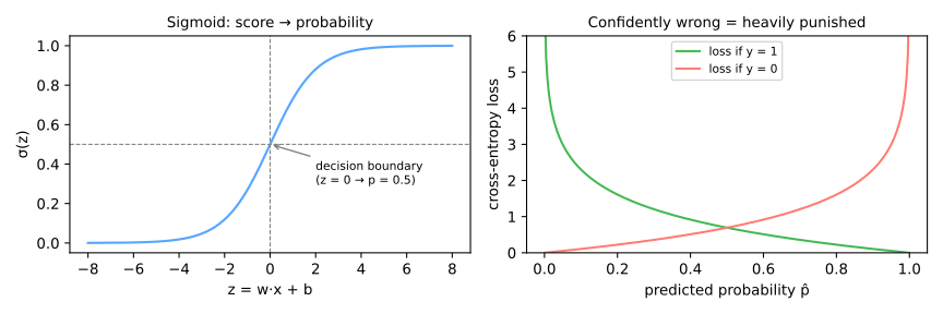
The top axis of the figure is the same curve read in hours: the steepest point, \(\hat p = 0.5\), is at \(-b/w = 6.75\) hours, and it takes less than two hours on either side to go from "almost surely fails" to "almost surely passes". The steepness is set by \(w\): a larger \(w\) makes a sharper transition.
The decision boundary is a line
With two features the score is \(z = w_1x_1 + w_2x_2 + b\), and the set of points where \(z = 0\) (probability exactly 0.5) is a straight line; with \(d\) features it is a hyperplane. That makes logistic regression a linear classifier: however the probabilities vary, the frontier between "predict 0" and "predict 1" is flat. Here are 200 points in two classes:
from sklearn.datasets import make_blobs

X2, y2 = make_blobs(n_samples=200, centers=[[-1, -0.5], [1, 1]], cluster_std=1.0, random_state=0)
clf = LogisticRegression(C=np.inf).fit(X2, y2)
w, b = clf.coef_[0], clf.intercept_[0]
print(f"w = {w.round(3)}   b = {b:.3f}   |w| = {np.linalg.norm(w):.3f}")

# walk away from the boundary along the direction of w, starting at two different points of it
u = w / np.linalg.norm(w)                              # unit vector perpendicular to the boundary
for start in [np.array([-b / w[0], 0.0]), np.array([0.0, -b / w[1]])]:
    pts = start + np.outer([-1, 0, 0.5, 1, 2], u)      # distances -1, 0, 0.5, 1, 2
    print(clf.predict_proba(pts)[:, 1].round(3))
print(sigmoid(np.linalg.norm(w) * np.array([-1, 0, 0.5, 1, 2])).round(3))
w = [1.832 1.371]   b = -0.266   |w| = 2.288
[0.092 0.5   0.758 0.908 0.99 ]
[0.092 0.5   0.758 0.908 0.99 ]
[0.092 0.5   0.758 0.908 0.99 ]
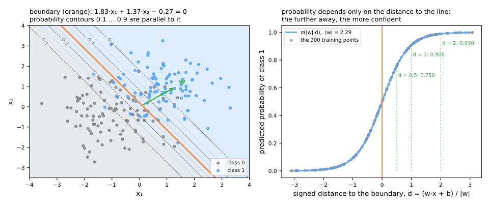
Two different starting points on the line, the same five distances, the same five probabilities: 0.092, 0.5, 0.758, 0.908, 0.99. The probability depends only on the signed distance \(d\) to the boundary, through \(\hat p = \sigma(\lVert w\rVert\, d)\), which is the third line of the output. Geometrically:
- the vector \(w\) is perpendicular to the boundary and points toward class 1 (the green arrow);
- the contours of equal probability are lines parallel to the boundary;
- \(\lVert w\rVert\) sets how fast confidence grows with distance. Here \(\lVert w\rVert = 2.29\), so one unit away from the line the model is already 90.8% sure.
Odds and interpretability
In linear regression each coefficient has a direct reading: one extra unit of \(x_j\) adds \(w_j\) to the prediction. In logistic regression \(w_j\) is still added to the score \(z\), but what happens to the probability? The answer appears once the probability is written another way: as odds.
The odds of an event are the probability that it happens divided by the probability that it does not, \(p/(1-p)\). It is the language of betting:
| probability \(p\) | odds \(p/(1-p)\) | in words |
|---|---|---|
| 0.75 | 0.75 / 0.25 = 3 | "3 to 1": out of 4 cases, 3 for and 1 against |
| 0.5 | 0.5 / 0.5 = 1 | "1 to 1": even |
| 0.2 | 0.2 / 0.8 = 0.25 | "1 to 4": out of 5 cases, 1 for and 4 against |
Probability runs from 0 to 1; odds run from 0 to infinity and equal 1 when \(p = 0.5\).
Now the link with the model. The predicted probability is \(\hat p = \sigma(z) = 1/(1+e^{-z})\), so the probability of the opposite is \(1 - \hat p = e^{-z}/(1+e^{-z})\). Dividing one by the other, the denominator \(1 + e^{-z}\) cancels:
The odds the model predicts are simply \(e^{z}\). Read from right to left, the same equality says the score \(z\) is the log of the odds, the logit (a name coined by Berkson in 1944, by analogy with Bliss's "probit"). The model is linear in the log-odds, not in the probability.
An example with numbers. Take a one-feature model with \(w = 0.8\) and \(b = -4\). For each value of \(x\) the table computes, from left to right: the score \(z = wx + b\); the predicted probability \(\hat p = \sigma(z)\), with the same sigmoid as before; the odds \(\hat p/(1-\hat p)\); and finally \(e^{z}\), to check the algebra above.
| \(x\) | score \(z = 0.8x - 4\) | probability \(\hat p = \sigma(z)\) | odds \(\hat p/(1-\hat p)\) | \(e^{z}\) |
|---|---|---|---|---|
| 4 | −0.8 | 0.310 | 0.449 | 0.449 |
| 5 | 0.0 | 0.500 | 1.000 | 1.000 |
| 6 | +0.8 | 0.690 | 2.226 | 2.226 |
The last two columns agree, as promised. Now compare the rows. Each extra unit of \(x\) adds 0.8 to the score; since the odds are \(e^{z}\), adding 0.8 to the exponent multiplies the odds by \(e^{0.8} = 2.226\). That is why the odds column goes from 0.449 to 1.000 to 2.226, each value 2.226 times the last. In general:
The probability follows no fixed rule. It grows 19 points from \(x=4\) to \(x=5\) and 19 again from 5 to 6, but that is a coincidence of the symmetry around 0.5; further from the center the jumps change size (the hours model just below shows it).
That is the honest sentence about a logistic coefficient: one extra unit of \(x_j\) multiplies the odds by \(e^{w_j}\), everywhere on the curve, holding the other features fixed. The change in probability depends on where you start: largest near \(p = 0.5\), vanishing in the tails. The same check on the fitted hours model:
print(f"e^w = {np.exp(model.coef_[0, 0]):.3f}")
odds = lambda p: p / (1 - p)
p = model.predict_proba([[5.0], [6.0], [7.0]])[:, 1]
print("p       ", p.round(3))
print("odds    ", odds(p).round(3))
print("ratios  ", (odds(p)[1:] / odds(p)[:-1]).round(3))
Each extra hour of study multiplies the odds of passing by 13.7. In probability that is +11 points from 5 to 6 hours, but +54 points from 6 to 7. The odds ratio \(e^{w}\) is the number doctors and credit analysts quote, and the reason logistic regression survives in regulated domains (Explainability). Two cautions carry over from linear regression: the reading assumes the other features are held fixed, and it compares coefficients fairly only when the features are on comparable scales (you will do it on standardized features in the lab).
The loss: cross-entropy
Stage 3. To fit \(w\) and \(b\) we need a number that measures how wrong the probabilities are. The principle is maximum likelihood: choose the parameters under which the labels we actually observed are as probable as possible. The probability the model gives to what happened to example \(i\) is \(\hat p_i\) if \(y_i = 1\) and \(1 - \hat p_i\) if \(y_i = 0\). Multiplying over the examples, taking the log (which turns the product into a sum), and flipping the sign so that smaller is better gives the log loss, or binary cross-entropy:
Only one of the two terms is alive for each example. Each term reads: minus the log of the probability the model gave to the truth.
By hand
Four predictions, two of each class:
| \(i\) | \(y\) | \(\hat p\) | probability given to the truth | \(-\ln(\cdot)\) |
|---|---|---|---|---|
| 1 | 1 | 0.9 | 0.9 | 0.105 |
| 2 | 1 | 0.6 | 0.6 | 0.511 |
| 3 | 0 | 0.3 | 0.7 | 0.357 |
| 4 | 0 | 0.8 | 0.2 | 1.609 |
The mean is \((0.105 + 0.511 + 0.357 + 1.609)/4 = 0.646\). The library agrees:
from sklearn.metrics import log_loss

y_true = np.array([1, 1, 0, 0])
p_hat = np.array([0.9, 0.6, 0.3, 0.8])
terms = -(y_true * np.log(p_hat) + (1 - y_true) * np.log(1 - p_hat))
print(terms.round(3), f"mean = {terms.mean():.3f}")
print(f"log_loss = {log_loss(y_true, p_hat):.3f}")
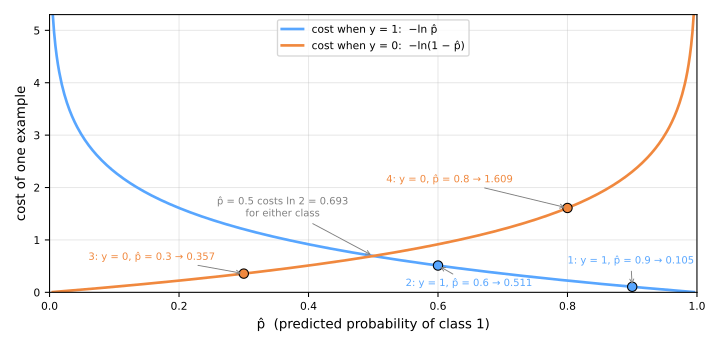
Point 4 is the only mistake, and a confident one (0.8 for the wrong class). It alone contributes 1.609 of the total 2.582, 62%. A timid correct answer (point 2, 0.6) costs 0.511; a confident correct one (point 1) costs 0.105. The loss rewards being right and being honest about how sure you are. Two reference values: a model that always says 0.5 scores \(\ln 2 = 0.693\), and a perfect model scores 0.
The figure draws the two terms of the sum as curves over \(\hat p\), with the four points of the table on them. For an example of class 1 only the blue curve counts, \(-\ln \hat p\); for class 0 only the orange one, \(-\ln(1 - \hat p)\). Each curve is 0 at the correct end and grows without bound at the wrong end: going from 0.8 to 0.99 for the wrong class takes the cost of point 4 from 1.609 to 4.6. The two curves cross at \(\hat p = 0.5\), where either class costs \(\ln 2\). The mean loss is just the average height of the dots.
Why not squared error?
Linear regression used squared error. Why not use \((y - \hat p)^2\) here? It is also small when \(\hat p\) is right and large when it is wrong. The reason is that, combined with the sigmoid, it fails in three ways. The figure sums up all three; each panel is then explained with numbers.
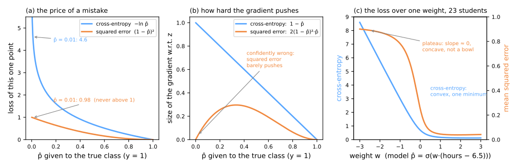
Panels (a) and (b) look at a single example of class 1 (\(y = 1\)) and vary the probability \(\hat p\) the model gives it; for class 0 everything is symmetric. Panel (c) looks at the average loss over a whole dataset.
(a) The price of a mistake. What that example costs under each loss:
| \(\hat p\) given to the true class | situation | squared error \((1-\hat p)^2\) | cross-entropy \(-\ln \hat p\) |
|---|---|---|---|
| 0.9 | confident and right | 0.010 | 0.105 |
| 0.5 | on the fence | 0.250 | 0.693 |
| 0.1 | wrong | 0.810 | 2.303 |
| 0.01 | badly wrong | 0.980 | 4.605 |
| 0.001 | very badly wrong | 0.998 | 6.908 |
Squared error never exceeds 1: to it, being wrong with \(\hat p = 0.1\) or with \(\hat p = 0.001\) costs almost the same (0.810 against 0.998). Cross-entropy tells the two apart (2.303 against 6.908): every extra factor of 10 of confidence in a mistake adds 2.3 to the loss.
(b) The push of the gradient. This is the main problem. Gradient descent fixes an example by moving its score \(z\). The strength of that fix is the derivative of the loss \(L\) with respect to \(z\). By the chain rule it has two factors:
The second factor is the slope of the sigmoid. It is almost zero on the flat parts of the curve, that is, whenever the model is very confident, right or wrong. For \(y = 1\):
- squared error: \(\partial L/\partial \hat p = -2(1-\hat p)\), so \(\partial L/\partial z = -2(1-\hat p)\cdot \hat p(1-\hat p)\). The sigmoid's slope stays in the product and, near \(\hat p = 0\), wipes out the gradient;
- cross-entropy: \(\partial L/\partial \hat p = -1/\hat p\), so \(\partial L/\partial z = -\frac{1}{\hat p}\cdot \hat p(1-\hat p) = -(1-\hat p) = \hat p - y\). The \(1/\hat p\) cancels the \(\hat p\) in the sigmoid's slope.
In numbers (the minus sign only says "increase \(z\)"; what matters is the size):
| \(\hat p\) given to the true class | sigmoid slope \(\hat p(1-\hat p)\) | \(\partial L/\partial z\), squared error | \(\partial L/\partial z\), cross-entropy |
|---|---|---|---|
| 0.5 | 0.25 | −0.250 | −0.500 |
| 0.1 | 0.09 | −0.162 | −0.900 |
| 0.01 | 0.0099 | −0.0196 | −0.990 |
| 0.001 | 0.001 | −0.0020 | −0.999 |
Read the squared-error column top to bottom: the worse the mistake, the weaker the push. At \(\hat p = 0.001\) it is 500 times weaker than cross-entropy's. The examples the model most needs to fix are exactly the ones squared error ignores. Cross-entropy does the opposite: the push grows with the mistake, up to a maximum of 1. Keep that factor \(\hat p(1-\hat p)\) in mind, which never exceeds 0.25: in neural networks, multiplied layer after layer, it is what wipes out the gradients of deep sigmoid networks. The last row, checked in code:
y1, p1 = 1, 0.001                                           # true class 1, model says 0.1%
print(f"d(MSE)/dz = {2 * (p1 - y1) * p1 * (1 - p1):.4f}   d(CE)/dz = {p1 - y1:.4f}")
(c) The shape of the loss. Now the average loss over the 23 students, as a function of one weight. To fit in a plot the model has a single parameter: \(\hat p = \sigma(w\,(\text{hours} - 6.5))\), with the hours centered at 6.5, close to the real boundary at 6.75 h. With \(w > 0\), more hours give a higher probability of passing: the right direction. With \(w < 0\), the model bets that whoever studies more fails; that is the wrong direction and nearly every student becomes a confident mistake.
x_c = hours - 6.5                                          # center the hours at 6.5
for wt in [-3, -1, 0, 1, 3]:
    p = sigmoid(wt * x_c)
    mse = np.mean((passed - p) ** 2)
    ce = -np.mean(passed * np.log(p) + (1 - passed) * np.log(1 - p))
    print(f"w = {wt:+d}   MSE = {mse:.3f}   cross-entropy = {ce:.3f}")
w = -3   MSE = 0.900   cross-entropy = 8.597
w = -1   MSE = 0.782   cross-entropy = 2.992
w = +0   MSE = 0.250   cross-entropy = 0.693
w = +1   MSE = 0.045   cross-entropy = 0.166
w = +3   MSE = 0.042   cross-entropy = 0.118
Picture gradient descent starting at \(w = -3\). With squared error the loss barely changes from \(w = -3\) to \(w = -1\) (from 0.900 to 0.782): the ground is a plateau, the slope is small and so are the steps. This is effect (b) summed over the 23 students, all confidently wrong. With cross-entropy the same stretch drops from 8.597 to 2.992: the slope is steep and points clearly the right way. There is also a guarantee. For logistic regression, cross-entropy is convex in \(w\) and \(b\): one valley, no local minima to get stuck in. Squared error is not convex (on the plateau the curve bends downward) and offers no such guarantee.
The simulator puts the two losses side by side on another small dataset. Move \(w\) and \(b\) and watch the right panel:
Training by gradient descent
There is no closed formula for the minimum of \(J\), as there was for least squares, so we walk down to it. The derivative is short. For one example, the chain rule through \(\hat p = \sigma(z)\) and \(\sigma'(z) = \sigma(z)(1-\sigma(z))\) gives
and since \(z = w^\top x + b\), the derivative with respect to \(w_j\) just multiplies by \(x_j\). Averaging over the examples:
This is the same shape as the linear regression gradient, \(X^\top(\text{prediction} - y)\), with \(\hat p = \sigma(Xw + b)\) in place of \(Xw\) (the factor 2 there comes from the square). Each example votes in proportion to how wrong its probability is. Each iteration of the loop has four stages, under the names they will get in neural networks:
- forward: compute the probabilities, \(\hat p = \sigma(Xw + b)\);
- loss: measure the cross-entropy \(J\);
- backward: compute the gradients \(\nabla_w J = \frac{1}{n}X^\top(\hat p - y)\) and \(\partial J/\partial b\);
- update: \(w \leftarrow w - \eta\,\nabla_w J\) and \(b \leftarrow b - \eta\,\partial J/\partial b\).
The gradient descent loop from the previous lesson, on the 200 points above:
w_gd, b_gd, eta = np.zeros(2), 0.0, 0.5
for it in range(2001):
    p = sigmoid(X2 @ w_gd + b_gd)
    if it in (0, 10, 100, 1000, 2000):
        loss = -np.mean(y2 * np.log(p) + (1 - y2) * np.log(1 - p))
        print(f"iter {it:4d}  loss {loss:.4f}  w {w_gd.round(4)}  b {b_gd:.4f}")
    w_gd -= eta * X2.T @ (p - y2) / len(y2)            # the gradient above
    b_gd -= eta * np.mean(p - y2)
print(f"sklearn          w {clf.coef_[0].round(4)}  b {clf.intercept_[0]:.4f}")
iter    0  loss 0.6931  w [0. 0.]  b 0.0000
iter   10  loss 0.3391  w [1.0142 0.6968]  b -0.0484
iter  100  loss 0.2956  w [1.7785 1.3219]  b -0.2455
iter 1000  loss 0.2955  w [1.8315 1.3718]  b -0.2663
iter 2000  loss 0.2955  w [1.8315 1.3718]  b -0.2663
sklearn          w [1.8317 1.3713]  b -0.2661
The loss starts at \(\ln 2 = 0.6931\) (all weights zero means \(\hat p = 0.5\) for everyone), falls fast in the first 10 steps, and stops changing at 0.2955 before iteration 1000. The weights agree with scikit-learn's to within 0.0005; the leftover is scikit-learn stopping as soon as its improvements fall below its tolerance (tol=1e-4). scikit-learn does not use this plain loop (its default lbfgs solver also uses curvature information and converges in a few steps, 7 in this example), but it minimizes the same function and lands in the same place, because a convex function has only one bottom. The stochastic version exists too: just as the previous lesson's SGDRegressor fits linear regression with SGD, SGDClassifier(loss='log_loss', penalty=None) fits this same logistic regression.
Curved boundaries: engineer the features
Stage 4. So far every boundary has been a straight line: the set of points where \(z = w_1x_1 + w_2x_2 + b = 0\). Many problems cannot be split by a line. The classic example is the circles: one class forms a small circle in the center and the other a larger circle around it. Any line leaves pieces of the outer circle on both sides.
The way out needs no new model. Logistic regression is linear in the features it receives, and those need not be the original measurements. If, instead of \(x_1\) and \(x_2\), it receives \(x_1^2\) and \(x_2^2\), the score becomes
and the boundary \(z = 0\) becomes \(w_1 x_1^2 + w_2 x_2^2 = -b\). With \(w_1\) and \(w_2\) negative and similar, that is a circle. It is the same idea as the polynomial features that let linear regression fit a parabola: the model stays linear in its features, but the boundary looks curved when drawn in the original measurements.
On data: 400 points, 200 on the inner circle (class 1) and 200 on the outer one (class 0), the inner radius half the outer, plus some noise. 30% of the points (120) are held out for testing:
from sklearn.datasets import make_circles
from sklearn.model_selection import train_test_split

X, y = make_circles(n_samples=400, noise=0.15, factor=0.5, random_state=0)   # class 1 = inner circle
X_a, X_b, y_a, y_b = train_test_split(X, y, test_size=0.3, stratify=y, random_state=0)

flat = LogisticRegression(C=np.inf).fit(X_a, y_a)                  # features x1, x2
circle = LogisticRegression(C=np.inf).fit(X_a ** 2, y_a)           # features x1², x2²
print(f"x1, x2      test {flat.score(X_b, y_b):.3f}")
print(f"x1², x2²    test {circle.score(X_b ** 2, y_b):.3f}   w = {circle.coef_[0].round(2)}   b = {circle.intercept_[0]:.2f}")
With \(x_1\) and \(x_2\), the line gets 40.0% of the test set right, worse than a coin: no line separates a circle from another one around it (landing below 50% is the luck of a 120-point sample). With \(x_1^2\) and \(x_2^2\), it gets 100%. The two weights came out almost equal (−16.83 and −16.00), so the model found on its own that the boundary is round: \(z = 0\) when \(16.8\,x_1^2 + 16.0\,x_2^2 = 9.70\), a circle of radius \(\sqrt{9.70/16.4} \approx 0.77\), between the inner circle (radius 0.5) and the outer one (radius 1). Inside it \(z > 0\): the model predicts class 1.
When the shape is not obvious. For the circles we knew in advance that the boundary was round. Usually we do not. The alternative is to generate all products of the measurements up to some degree at once, with PolynomialFeatures. With two measurements and degree 3 that is 9 features: \(x_1, x_2, x_1^2, x_1x_2, x_2^2, x_1^3, x_1^2x_2, x_1x_2^2, x_2^3\). The boundary \(z = 0\) can then be any degree-3 curve. The test below compares the line with this version on two shapes: the circles and the moons, two half-moons interlocked with each other (also 400 points, 30% for testing):
from sklearn.datasets import make_moons
from sklearn.pipeline import make_pipeline
from sklearn.preprocessing import PolynomialFeatures, StandardScaler

for name, (X, y) in [('moons', make_moons(n_samples=400, noise=0.2, random_state=0)),
                     ('circles', make_circles(n_samples=400, noise=0.15, factor=0.5, random_state=0))]:
    X_a, X_b, y_a, y_b = train_test_split(X, y, test_size=0.3, stratify=y, random_state=0)
    plain = make_pipeline(StandardScaler(), LogisticRegression(C=np.inf)).fit(X_a, y_a)
    poly = make_pipeline(PolynomialFeatures(degree=3, include_bias=False), StandardScaler(),
                         LogisticRegression(C=np.inf, max_iter=5000)).fit(X_a, y_a)
    print(f"{name:8s} plain: test {plain.score(X_b, y_b):.3f}   "
          f"degree 3 ({poly[0].n_output_features_} features): test {poly.score(X_b, y_b):.3f}")
moons    plain: test 0.917   degree 3 (9 features): test 0.958
circles  plain: test 0.400   degree 3 (9 features): test 0.958
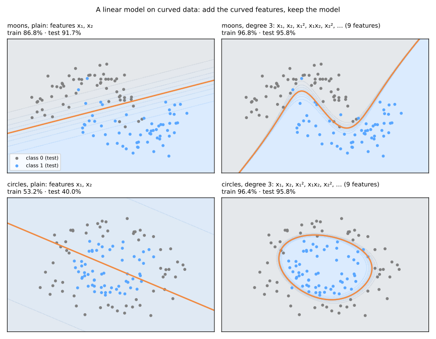
On the moons a line already does reasonably well (91.7%), because only the tips of the half-moons interlock; the degree-3 curve bends around the tips and reaches 95.8%. On the circles the 9 generic features also solve the problem (95.8%) but fall short of the 2 right features (100%). When you know the shape, building the right feature beats generating many.
Note the StandardScaler after PolynomialFeatures. On the moons \(x_1\) runs from −1.35 to 2.4, but \(x_1^3\) runs from −2.4 to 13.8. Features on such different scales stretch the loss landscape, and gradient-based solvers walk slowly down it. Standardizing after expanding puts every feature on the same scale.
The model is still an ordinary logistic regression, just with 9 features: cross-entropy, convexity and the gradient all work as before. There are two prices. The first is interpretation: the reading "one extra unit of \(x_j\), holding the others fixed" loses its meaning, because \(x_1^2\) cannot change unless \(x_1\) changes too. The second is overfitting: more features mean more capacity to overfit, as you saw in the previous lesson. When not even polynomials capture the shape of the boundary, it is time for models that find it on their own: k-NN in the next lesson, and later trees and neural networks.
Multi-class: softmax
For \(k\) classes the model learns one weight vector and one intercept per class, giving \(k\) scores \(z_c = w_c^\top x + b_c\). The softmax turns the scores into probabilities that are positive and sum to 1:
By hand
Three scores \(z = (2.0,\ 1.0,\ 0.1)\):
| class | \(z_c\) | \(e^{z_c}\) | \(\hat p_c = e^{z_c} / 11.212\) |
|---|---|---|---|
| A | 2.0 | 7.389 | 0.659 |
| B | 1.0 | 2.718 | 0.242 |
| C | 0.1 | 1.105 | 0.099 |
| sum | 11.212 | 1.000 |
The largest score wins, but not by everything: a gap of 1 in score is a factor \(e \approx 2.7\) in probability. Adding the same constant to all scores changes nothing (it multiplies numerator and denominator by the same \(e^c\)), which is why code subtracts the largest score before exponentiating, to avoid overflow. With two classes, softmax is the sigmoid: \(e^{z_1}/(e^{z_0}+e^{z_1}) = \sigma(z_1 - z_0)\).
With scikit-learn, on wine
The wine dataset: 178 wines from three cultivars (grape varieties) of the same Italian region, each described by 13 chemical measurements. To keep the example small we use two of them, alcohol and flavanoids. LogisticRegression switches to softmax by itself when \(y\) has more than two classes:
from sklearn.datasets import load_wine

def softmax(z):
    e = np.exp(z - z.max(axis=1, keepdims=True))       # subtract the max: same result, no overflow
    return e / e.sum(axis=1, keepdims=True)

wine = load_wine()
cols = [wine.feature_names.index(c) for c in ['alcohol', 'flavanoids']]
Xw, yw = wine.data[:, cols], wine.target
wine_model = make_pipeline(StandardScaler(), LogisticRegression(C=np.inf)).fit(Xw, yw)
print(wine.target_names, "coef_:", wine_model[-1].coef_.shape, "intercept_:", wine_model[-1].intercept_.shape)

picks = [0, 100, 133]                                  # one wine of each cultivar
z = wine_model.decision_function(Xw[picks])            # 3 scores per wine
print("true cultivar", yw[picks])
print("scores\n", z.round(2))
print("softmax\n", softmax(z).round(3))
print("predict_proba\n", wine_model.predict_proba(Xw[picks]).round(3))
print("predict      ", wine_model.predict(Xw[picks]))
P = wine_model.predict_proba(Xw)
print(f"rows sum to 1: {np.allclose(P.sum(axis=1), 1)}   "
      f"max |predict_proba - softmax|: {np.abs(P - softmax(wine_model.decision_function(Xw))).max()}")
['class_0' 'class_1' 'class_2'] coef_: (3, 2) intercept_: (3,)
true cultivar [0 1 2]
scores
 [[ 6.47 -0.22 -6.25]
 [-0.29  5.32 -5.02]
 [-3.11  1.56  1.55]]
softmax
 [[0.999 0.001 0.   ]
 [0.004 0.996 0.   ]
 [0.005 0.502 0.493]]
predict_proba
 [[0.999 0.001 0.   ]
 [0.004 0.996 0.   ]
 [0.005 0.502 0.493]]
predict       [0 1 1]
rows sum to 1: True   max |predict_proba - softmax|: 0.0
coef_ has shape (3, 2): one row of 2 weights per cultivar, plus 3 intercepts. predict_proba is exactly softmax(decision_function), and every row sums to 1. The three wines are instructive. Wine 0 is cultivar 0 with 0.999, easy. Wine 100 is cultivar 1 with 0.996. Wine 133 belongs to cultivar 2, but its scores for cultivars 1 and 2 are almost tied (1.56 and 1.55), so the model splits it 0.502 / 0.493 and predict gets it wrong, by a hair. The probabilities say how ambiguous, which a bare label cannot.
The loss is the same cross-entropy, \(-\ln \hat p_{\text{true class}}\), averaged. Wine 0 costs \(-\ln 0.999 \approx 0.001\); wine 133, whose true cultivar got only 0.493, costs \(-\ln 0.493 \approx 0.706\), seven hundred times more. This exact construction (linear scores, softmax, cross-entropy) is the output layer of essentially every neural classifier, including the language models that choose the next token among tens of thousands.
From probabilities to labels: the threshold
Stage 5. predict is predict_proba plus a threshold of 0.5 (for two classes; for several, the class with the largest probability). The 0.5 is a choice, not part of the model. Moving it trades one kind of mistake for the other, on the 200 points from before:
p_hat = clf.predict_proba(X2)[:, 1]
print("predict == (p >= 0.5):", np.array_equal(clf.predict(X2), (p_hat >= 0.5).astype(int)))
for t in [0.2, 0.5, 0.8]:
    pred = (p_hat >= t).astype(int)
    print(f"threshold {t}: class 1 predicted {pred.sum():3d} times · missed class 1: "
          f"{((pred == 0) & (y2 == 1)).sum():2d} · false alarms: {((pred == 1) & (y2 == 0)).sum():2d}"
          f" · accuracy {np.mean(pred == y2):.3f}")
predict == (p >= 0.5): True
threshold 0.2: class 1 predicted 131 times · missed class 1:  1 · false alarms: 32 · accuracy 0.835
threshold 0.5: class 1 predicted  97 times · missed class 1: 12 · false alarms:  9 · accuracy 0.895
threshold 0.8: class 1 predicted  76 times · missed class 1: 31 · false alarms:  7 · accuracy 0.810
Lowering the threshold to 0.2 misses almost no class-1 point (1 instead of 12) and pays with 32 false alarms instead of 9; raising it to 0.8 does the opposite. Accuracy is best at 0.5 here, but accuracy counts both mistakes as equally bad. When a missed cancer is worse than a false alarm, or the positive class is rare, that is the wrong criterion, and the threshold should move. How to measure the two kinds of mistake and choose the threshold is the subject of Classification Metrics and ROC & PR curves. Logistic regression's contribution is to give you probabilities worth thresholding.
Practical profile
| Strengths | fast to train and to predict; convex loss (the same answer every time, no initialization luck); probabilities that are usually reasonable out of the box; interpretable through odds ratios; a strong baseline that scales to millions of rows |
| Weaknesses | linear boundary (curves need engineered features); interactions between features must be added by hand; slow to converge on unscaled features; coefficients of correlated features are unstable to read, even when predictions are fine |
| Watch out for | max_iter warnings usually mean unscaled features; one-hot columns for every category next to an intercept leave single coefficients meaningless (drop a reference category); odds ratios are not probability ratios |
| Reach for it when | you need a solid, explainable baseline; probabilities matter (risk, triage, ranking); features are informative on their own |
Lab: predicting survival on the Titanic
The Titanic passenger list from the preprocessing lesson, now with a question: who survived? It exercises everything above on real, messy data: a pipeline with imputation, encoding and scaling; probabilities checked by hand; coefficients read as odds ratios; and an honest estimate of accuracy on passengers the model never saw. The model is the plain logistic regression of this lesson (C=np.inf), so there is nothing to tune: we split the data once into train (fit and study the model) and test (report, once, at the end).
How to run this lab in class (about 60 min, in pairs)
- Open the lab notebook in Colab and save a copy to your Drive (File → Save a copy in Drive) before editing. Run the cells in order, in one session.
- Each step starts with a Predict: answer it with your partner before running the cell. Getting the prediction wrong is what makes the result stick.
- After running, compare with the output and the reading on this page. Every output here is exactly what the code prints.
- The Simulations ask you to write a small Python experiment: change one input of the model and watch what happens to the output. No arithmetic by hand. The solution is collapsed right below: try before opening it.
- Suggested pace: steps 1 to 4 in 20 min; steps 5 to 7 in 25 min; step 8 and the wrap-up in 15 min. Your turn is homework.
Step 1 — load and look
Predict. Is the overall survival rate above or below 50%? Who survived more: third-class women or first-class men?
import numpy as np
import pandas as pd

url = "https://raw.githubusercontent.com/hsandmann/biblio/refs/heads/main/ml/aula04/titanic/train.csv"
df = pd.read_csv(url)
print(df.shape)
print(f"survival rate: {df['Survived'].mean():.3f}")
print(df.pivot_table(index='Sex', columns='Pclass', values='Survived', aggfunc='mean').round(3))
print("missing:", df[['Age', 'Embarked', 'Cabin']].isna().sum().to_dict())
(891, 12)
survival rate: 0.384
Pclass      1      2      3
Sex
female  0.968  0.921  0.500
male    0.369  0.157  0.135
missing: {'Age': 177, 'Embarked': 2, 'Cabin': 687}
891 passengers, 38.4% survived. The table is survival rate by sex and ticket class, and it already tells most of the story: 96.8% of first-class women survived, 13.5% of third-class men. Two things to notice for later. Sex and class both matter, and they interact: for women, going from 2nd to 3rd class costs 42 points (0.921 → 0.500); for men, 2 points (0.157 → 0.135). A logistic regression with only Sex and Pclass columns cannot represent that on its own (see Your turn). And Age is missing for 177 passengers, Embarked for 2, Cabin for 687; we will impute the first two and leave Cabin out.
Step 2 — train and test
Predict. Why set the test set aside now, before building any model? Why not leave it for the end?
from sklearn.model_selection import train_test_split

features = ['Pclass', 'Sex', 'Age', 'SibSp', 'Parch', 'Fare', 'Embarked']
X, y = df[features], df['Survived']
X_train, X_test, y_train, y_test = train_test_split(X, y, test_size=0.2, stratify=y, random_state=42)
print(len(X_train), len(X_test))
print(f"survival rate: train {y_train.mean():.3f} · test {y_test.mean():.3f}")
80% of the passengers (712) go to training and 20% (179) to the test set, which is not touched again until step 8. stratify keeps the survival rate at 38% in both parts. Features are the seven raw columns; Name, Ticket, Cabin and PassengerId are left out. There is no validation set because there is nothing to choose: the plain model has no knob to tune. (When there is one, you carve a validation split out of the training rows, or use the cross-validation you will meet later in the course.)
Step 3 — a baseline
Predict. Is a "model" that always answers "did not survive", without looking at the passenger, right more or less than half of the time? Why?
from sklearn.dummy import DummyClassifier

dummy = DummyClassifier(strategy='most_frequent').fit(X_train, y_train)
print(f"always 'did not survive': train accuracy {dummy.score(X_train, y_train):.3f}")
A "model" that ignores the passenger and always answers the majority class ("did not survive") is right 61.7% of the time on the training set. That is the floor. Any accuracy we report means something only in comparison to it; in step 8 both are measured on the test set.
Step 4 — the pipeline
Predict. Pclass is 1, 2 or 3. Why treat it as a category (one one-hot column per class) rather than as a number?
from sklearn.compose import ColumnTransformer
from sklearn.impute import SimpleImputer
from sklearn.linear_model import LogisticRegression
from sklearn.pipeline import make_pipeline
from sklearn.preprocessing import OneHotEncoder, StandardScaler

numeric = ['Age', 'SibSp', 'Parch', 'Fare']
categorical = ['Pclass', 'Sex', 'Embarked']

preprocess = ColumnTransformer([
    ('num', make_pipeline(SimpleImputer(strategy='median'), StandardScaler()), numeric),
    ('cat', make_pipeline(SimpleImputer(strategy='most_frequent'),
                          OneHotEncoder(drop='first')), categorical)])
model = make_pipeline(preprocess, LogisticRegression(C=np.inf, max_iter=1000))   # C=np.inf: no penalty
model.fit(X_train, y_train)

enc = model[0].named_transformers_['cat'][-1]
print("reference (dropped) categories:", {c: cats[0] for c, cats in zip(categorical, enc.categories_)})
print(f"{model[-1].coef_.size} coefficients · train accuracy {model.score(X_train, y_train):.3f}")
reference (dropped) categories: {'Pclass': 1, 'Sex': 'female', 'Embarked': 'C'}
9 coefficients · train accuracy 0.809
The ColumnTransformer sends each column through its own treatment: numbers get the median for missing values and are then standardized; categories get the most frequent value and are one-hot encoded. Pclass is treated as a category, with no assumption that 2nd class is exactly "halfway" between 1st and 3rd. Everything is fitted on the training rows only, inside the pipeline.
Why drop='first'. If the encoder kept one column per category, every passenger would have exactly one 1 among Pclass_1, Pclass_2 and Pclass_3: the three columns would always add up to 1, exactly like the constant column that the intercept multiplies. Adding 5 to the three class weights and subtracting 5 from the intercept would then give the same predictions, so the model would have infinitely many equally good sets of weights and no single one-hot coefficient would mean anything. Dropping the first category of each variable removes the redundancy. The dropped categories are the reference, printed on the first line: a first-class woman who boarded at Cherbourg. Every remaining one-hot coefficient is read relative to that reference (step 7). That leaves 9 coefficients: 4 numeric, 2 for class, 1 for sex, 2 for the port.
The model gets 80.9% of the training passengers right, against 61.7% for the baseline. Training accuracy is optimistic (these passengers were used to fit the weights), but with 9 coefficients for 712 passengers there is little room to overfit; step 8 will measure how optimistic it was.
Step 5 — probabilities for two passengers
Predict. Looking at the table of step 1: a third-class man and a first-class woman. Who gets a high probability and who gets a low one?
passengers = pd.DataFrame({'Pclass': [3, 1], 'Sex': ['male', 'female'], 'Age': [25, 30],
                           'SibSp': [0, 1], 'Parch': [0, 0], 'Fare': [8.05, 80.0],
                           'Embarked': ['S', 'C']})
print(model.predict_proba(passengers).round(3))
print(model.predict(passengers))
Two invented passengers: a 25-year-old man traveling alone in third class on an 8-pound ticket from Southampton, and a 30-year-old woman in first class with her husband, on an 80-pound ticket from Cherbourg. Each row of predict_proba is (did not survive, survived) and sums to 1. The model gives him 9.3% and her 94.2%, in line with the table of step 1.
Simulation: the effect of age. Take a second-class passenger traveling with his parents (Parch = 2) and a sibling (SibSp = 1), on a 30-pound ticket from Southampton. Change only the age (2, 8, 15, 25, 40 and 60 years), first for a boy and then for a girl. Watch the predicted probability. Then check in the training rows how many second-class children aged 12 or under survived.
Solution
ages = [2, 8, 15, 25, 40, 60]
print("age    ", ages)
for sex in ['male', 'female']:
    people = pd.DataFrame({'Pclass': 2, 'Sex': sex, 'Age': ages, 'SibSp': 1, 'Parch': 2,
                           'Fare': 30.0, 'Embarked': 'S'})
    print(f"{sex:7s}", model.predict_proba(people)[:, 1].round(3))

train = df.loc[X_train.index]                        # training rows only
kids = train[(train['Age'] <= 12) & (train['Pclass'] == 2)]
print(kids.groupby('Sex')['Survived'].agg(['mean', 'size']))
age     [2, 8, 15, 25, 40, 60]
male    [0.38  0.326 0.268 0.198 0.12  0.059]
female  [0.9   0.876 0.843 0.784 0.667 0.477]
        mean  size
Sex
female   1.0     7
male     1.0     8
To the model, age has the same effect on everyone: the probability falls smoothly with the years, for boys and for girls. The 8-year-old boy gets only 32.6%. In the training data, however, all 15 second-class children aged 12 or under survived, boys included. The rule "women and children first" is an interaction between age and sex: being a child changes a boy's fate a lot and a girl's only a little. A logistic regression can only represent it if someone builds the feature that describes it; exercise 1 of Your turn does that for another interaction, between sex and class.
Step 6 — the man's probability, by hand
Predict. Which feature do you expect to pull the man's score down the most?
names = model[0].get_feature_names_out()
w, b = model[-1].coef_[0], model[-1].intercept_[0]
x_man = model[0].transform(passengers)[0]            # the 3rd-class man, after preprocessing
print(pd.DataFrame({'x': x_man, 'w': w, 'w*x': w * x_man}, index=names).round(3))
z = b + (w * x_man).sum()
print(f"z = {b:.3f} + {(w * x_man).sum():.3f} = {z:.3f}   sigmoid(z) = {1 / (1 + np.exp(-z)):.3f}")
                     x      w    w*x
num__Age        -0.350 -0.513  0.180
num__SibSp      -0.465 -0.267  0.124
num__Parch      -0.466 -0.072  0.034
num__Fare       -0.495  0.108 -0.053
cat__Pclass_2    0.000 -0.987 -0.000
cat__Pclass_3    1.000 -2.239 -2.239
cat__Sex_male    1.000 -2.685 -2.685
cat__Embarked_Q  0.000  0.320  0.000
cat__Embarked_S  1.000 -0.417 -0.417
z = 2.782 + -5.057 = -2.275   sigmoid(z) = 0.093
This is the whole model, laid open. The column x is what the classifier actually sees: the four numbers standardized (age 25 is 0.350 standard deviations below the training mean, so \(-0.350\)) and a 1 in the column of each non-reference category he belongs to: third class, male, Southampton. Multiply by the weights, add, add the intercept: \(z = -2.275\). Then \(\sigma(-2.275) = 0.093\), the 9.3% of step 5.
With a reference category the intercept has a reading of its own: \(b = 2.782\) is the log-odds of the reference passenger, a first-class woman from Cherbourg with average age, family and fare, whose probability is \(\sigma(2.782) = 0.942\). Starting from her, being a man subtracts 2.685 from the score, third class 2.239 and Southampton 0.417. His youth helps a little (+0.180, because the age coefficient is negative and he is younger than average), and so does traveling alone (+0.124).
Simulation: one feature at a time. Start from the third-class man and turn him, one step at a time, into the reference passenger: first change the sex to female, then the class to 1, then the port to C. At each step, print the score \(z\) (model.decision_function) and the probability. How much does \(z\) change at each step? And the probability?
Solution
step = passengers.iloc[[0]].copy()                  # start from the third-class man
z_old, p_old = model.decision_function(step)[0], model.predict_proba(step)[0, 1]
print(f"{'start':22s} z = {z_old:+.3f}             p = {p_old:.3f}")
for col, val in [('Sex', 'female'), ('Pclass', 1), ('Embarked', 'C')]:
    step[col] = val
    z, p = model.decision_function(step)[0], model.predict_proba(step)[0, 1]
    print(f"{col + ' -> ' + str(val):22s} z = {z:+.3f} ({z - z_old:+.3f})   p = {p:.3f} ({p - p_old:+.3f})")
    z_old, p_old = z, p
start                  z = -2.275             p = 0.093
Sex -> female          z = +0.410 (+2.685)   p = 0.601 (+0.508)
Pclass -> 1            z = +2.649 (+2.239)   p = 0.934 (+0.333)
Embarked -> C          z = +3.066 (+0.417)   p = 0.955 (+0.022)
Each change adds exactly its coefficient to the score (2.685, 2.239 and 0.417, the numbers in the table above), wherever you start. The probability does not behave that way: the same change is worth a lot near 0.5 and almost nothing near 1. Switching the port adds 0.417 to the score but only 2 points to the probability, because it was already at 0.934, on the flat part of the sigmoid.
Step 7 — coefficients as odds ratios
Predict. The Age coefficient is negative. So, holding the rest fixed, does an older passenger have higher or lower odds of surviving? Is its odds ratio \(e^{\text{coef}}\) above or below 1?
coef = pd.Series(w, index=names)
print(pd.DataFrame({'coef': coef, 'e^coef': np.exp(coef)}).round(3))
sd = model[0].named_transformers_['num'][-1].scale_
print("one standard deviation:", ", ".join(f"{c} {s:.1f}" for c, s in zip(numeric, sd)))
                  coef  e^coef
num__Age        -0.513   0.599
num__SibSp      -0.267   0.765
num__Parch      -0.072   0.931
num__Fare        0.108   1.114
cat__Pclass_2   -0.987   0.373
cat__Pclass_3   -2.239   0.107
cat__Sex_male   -2.685   0.068
cat__Embarked_Q  0.320   1.377
cat__Embarked_S -0.417   0.659
one standard deviation: Age 13.0, SibSp 1.1, Parch 0.8, Fare 48.0
Numeric features are standardized, so each coefficient is per one standard deviation, printed on the last line. Age: \(e^{-0.513} = 0.599\), so 13.0 more years of age multiply the odds of survival by 0.599 (about 40% lower odds), with sex, class, fare and the rest held fixed. Fare: one standard deviation (48.0 pounds) multiplies the odds by 1.114.
One-hot features compare their category with the reference category of the same variable, everything else held fixed. Sex_male = -2.685: a man has \(e^{-2.685} = 0.068\) times the odds of survival of a woman with the same class, age, family, fare and port. Pclass_3 = -2.239: a third-class passenger has 0.107 times the odds of an otherwise identical first-class one; second class, 0.373 times. Embarked_S: a passenger who boarded at Southampton has 0.659 times the odds of one who boarded at Cherbourg. To read a comparison the other way round, flip the sign (and invert the odds ratio); to compare two categories that are not the reference, subtract their coefficients:
print(f"woman vs man:      odds x {np.exp(-coef['cat__Sex_male']):.2f}")
print(f"1st vs 3rd class:  odds x {np.exp(-coef['cat__Pclass_3']):.2f}")
print(f"2nd vs 3rd class:  odds x {np.exp(coef['cat__Pclass_2'] - coef['cat__Pclass_3']):.2f}")
A woman has 14.7 times the odds of survival of a man with the same class, age, fare, family and port. A first-class passenger has 9.4 times the odds of an otherwise identical third-class one, and a second-class passenger 3.5 times. These are the numbers to report. Which category is the reference is a choice of presentation: another choice changes the coefficients but not a single prediction. And odds ratios are not probability ratios: 14.7 times the odds is not 14.7 times the probability, which cannot exceed 1.
Simulation: the odds ratio is the same for everyone. Take three different passengers (the third-class man, a 30-year-old first-class man and the boy of the step 5 simulation). For each one, use predict_proba to get the probability as a woman and as a man, keeping everything else. Compare the ratio of the probabilities with the ratio of the odds.
Solution
odds = lambda p: p / (1 - p)
people = pd.DataFrame({'Pclass': [3, 1, 2], 'Sex': 'male', 'Age': [25, 30, 8], 'SibSp': [0, 1, 1],
                       'Parch': [0, 0, 2], 'Fare': [8.05, 80.0, 30.0], 'Embarked': ['S', 'C', 'S']})
for i in range(len(people)):
    one = people.iloc[[i]]
    p_f = model.predict_proba(one.assign(Sex='female'))[0, 1]
    p_m = model.predict_proba(one.assign(Sex='male'))[0, 1]
    print(f"p woman {p_f:.3f} · p man {p_m:.3f} · probability ratio {p_f / p_m:5.2f}"
          f" · odds ratio {odds(p_f) / odds(p_m):.2f}")
p woman 0.601 · p man 0.093 · probability ratio  6.45 · odds ratio 14.66
p woman 0.942 · p man 0.523 · probability ratio  1.80 · odds ratio 14.66
p woman 0.876 · p man 0.326 · probability ratio  2.69 · odds ratio 14.66
The odds ratio comes out 14.66 for all three, exactly the \(e^{2.685}\) of the table: it is the one number that describes the effect of sex for any passenger. The probability ratio changes from passenger to passenger (from 1.80 to 6.45), because it depends on where each one starts. That is why the odds ratio is what gets reported.
Step 8 — the one and only test
Predict. Will test accuracy land above or below the 80.9% on training? By a lot or a little?
from sklearn.metrics import confusion_matrix

print(f"test accuracy {model.score(X_test, y_test):.3f} · baseline {dummy.score(X_test, y_test):.3f}")
print(confusion_matrix(y_test, model.predict(X_test), labels=[1, 0]))   # positive first
Only now do we touch the test set: 80.4% accuracy against 61.5% for the baseline, close to the 80.9% on training, so the training number was only slightly optimistic. The 2×2 table is a first look at the confusion matrix: rows are the truth (survived, died), columns the prediction, positive class first: the standard layout, [[TP, FN], [FP, TN]], which labels=[1, 0] asks scikit-learn for. Of the 69 survivors in the test set, the model missed 23; of the 110 who died, it wrongly called 12 survivors. Accuracy mixes these two kinds of mistake into one number, and the next lessons take them apart.
If 80.4% disappoints you and you go back to step 4 to try other features, the test set becomes part of your design loop and 80.4% stops meaning anything. Compare variants on a validation split carved out of the training rows (as in Your turn), and keep the test for the end.
Simulation: moving the threshold. predict uses a threshold of 0.5. On the training rows (the test set is spent), classify with thresholds 0.3, 0.4, 0.5, 0.6 and 0.7 and print, for each, the fraction of survivors found, the fraction of deaths recognized and the accuracy.
Solution
p_train = model.predict_proba(X_train)[:, 1]         # on training rows: the test set is spent
for t in [0.3, 0.4, 0.5, 0.6, 0.7]:
    pred = (p_train >= t).astype(int)
    found = pred[y_train == 1].mean()                # fraction of survivors found
    recog = 1 - pred[y_train == 0].mean()            # fraction of deaths recognized
    print(f"threshold {t}: survivors found {found:.3f} · deaths recognized {recog:.3f}"
          f" · accuracy {(pred == y_train).mean():.3f}")
threshold 0.3: survivors found 0.824 · deaths recognized 0.745 · accuracy 0.775
threshold 0.4: survivors found 0.751 · deaths recognized 0.804 · accuracy 0.784
threshold 0.5: survivors found 0.714 · deaths recognized 0.868 · accuracy 0.809
threshold 0.6: survivors found 0.652 · deaths recognized 0.916 · accuracy 0.815
threshold 0.7: survivors found 0.553 · deaths recognized 0.964 · accuracy 0.806
Lowering the threshold finds more survivors and recognizes fewer deaths; raising it does the opposite. Accuracy barely moves (from 0.775 to 0.815) and hides that trade. Which threshold is best depends on which mistake costs more, not on accuracy; the two fractions have names (recall and specificity) and are the subject of Classification Metrics.
To close the class. One sentence each: (1) what does a logistic regression coefficient multiply? (2) Why did the boy of the step 5 simulation get such a low probability? (3) Why can the test set be used only once?
Your turn
For homework, with more time:
- The interaction. Step 1 showed that third class hurts women far more than men. Add a column
df['female_3rd'] = ((df['Sex'] == 'female') & (df['Pclass'] == 3)).astype(int), put it infeaturesand incategorical(withdrop='first'its coefficient compares 1 with 0) and redo steps 2 to 7. Read its odds ratio in words. How does theSex_malecoefficient change, and why? To decide whether the column helps, splitX_trainagain into a training and a validation part and compare the two models there, not on the test set. - The threshold. On such a validation split, compute
p = model.predict_proba(X_val)[:, 1]and count the survivors missed and the false alarms for thresholds 0.3, 0.5 and 0.7. Which threshold would you use if a missed survivor were three times worse than a false alarm? - Why a reference category. Build the pipeline again with
OneHotEncoder()(nodrop) and fit it. Then add 5 to the threePclassweights inmodel[-1].coef_and subtract 5 frommodel[-1].intercept_: do the predicted probabilities onX_testchange? What does that say about reading a single coefficient when every category keeps its column? - From scratch. Take
Xt = model[0].transform(X_train)and run the gradient-descent loop of this lesson (weights and intercept, \(\eta = 0.5\)). Compare withmodel[-1].coef_andmodel[-1].intercept_. After how many iterations do they agree to two decimals?
References
- Verhulst, P.-F. "Notice sur la loi que la population suit dans son accroissement." Correspondance Mathématique et Physique 10 (1838), 113–121. full text
- Berkson, J. "Application of the Logistic Function to Bio-Assay." Journal of the American Statistical Association 39, no. 227 (1944): 357–365 — coins the word logit. DOI
- Cox, D. R. "The Regression Analysis of Binary Sequences." JRSS B 20 (1958). DOI