Machine Learning · Insper

Logistic Regression

Advanced approach

Why cross-entropy and not squared error, and how the same model goes beyond a straight line and beyond two classes

The path of this part

Why cross-entropythe price, the push and the shape of the loss
Curved boundariessquared and polynomial features
Many classessoftmax, on wine
Use it wellstrengths, weaknesses, traps

Each stage answers one question: why not keep the squared error of linear regression? → what if no line separates the classes? → what if there are more than two classes? → when is logistic regression the right tool?

Stage 1 · why not keep the squared error of linear regression?

Why not squared error?

\((y - \hat p)^2\) is also small when the predicted probability \(\hat p\) is right and large when it is wrong. Predict. Combined with the sigmoid, what could go wrong?

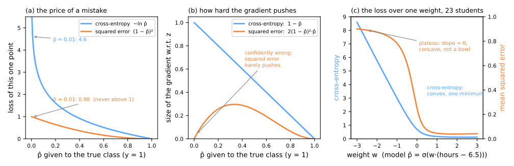
(a) cross-entropy grows without bound, squared error never exceeds 1; (b) cross-entropy pushes hardest on the worst mistakes; (c) cross-entropy is one convex valley, squared error has a plateau

(a) the price

squared error never exceeds 1: \(\hat p = 0.1\) and \(0.001\) cost 0.810 and 0.998; cross-entropy, 2.303 and 6.908

(b) the push

the worse the mistake, the weaker the squared-error gradient

(c) the shape

cross-entropy is convex; squared error has a plateau

(b) The push of the gradient

\(L\): the loss of one example of class 1 (\(y = 1\)). Gradient descent fixes it by moving its score \(z\); the strength is, by the chain rule, \(\partial L/\partial z = \partial L/\partial \hat p \cdot \hat p(1-\hat p)\), where \(\hat p(1-\hat p)\) is the slope of the sigmoid:

\[ \text{squared error: } -2(1-\hat p)\cdot\hat p(1-\hat p) \qquad \text{cross-entropy: } -\tfrac{1}{\hat p}\cdot\hat p(1-\hat p) = \hat p - y \]

\(\hat p\) given to the true class	sigmoid slope	squared error	cross-entropy
0.5	0.25	−0.250	−0.500
0.1	0.09	−0.162	−0.900
0.01	0.0099	−0.0196	−0.990
0.001	0.001	−0.0020	−0.999

With squared error the examples most in need of fixing are the ones it ignores (500 times weaker at 0.001). Cross-entropy's \(1/\hat p\) cancels the sigmoid's slope.

(c) The shape of the loss

One weight, \(\hat p = \sigma(w\,(\text{hours} - 6.5))\), on the 23 students: average loss over all of them. \(w < 0\) bets that whoever studies more fails.

\(w\)	−3	−1	0	+1	+3
squared error	0.900	0.782	0.250	0.045	0.042
cross-entropy	8.597	2.992	0.693	0.166	0.118

Panel (c): cross-entropy is one convex valley over the weight; squared error has a plateau when the weight points the wrong way

From \(w = -3\) squared error is a plateau (0.900 → 0.782); cross-entropy drops steeply (8.597 → 2.992). And it is convex: one valley, no local minima.

Simulator: the two losses side by side

Predict. Turn \(w\) the wrong way. Which loss notices that something is badly wrong?

Stage 2 · what if no line separates the classes?

Curved boundaries: engineer the features

The circles: one class inside, the other around it. Any line leaves pieces of the outer circle on both sides.

Predict. Give logistic regression \(x_1^2\) and \(x_2^2\) instead of \(x_1\) and \(x_2\). What shape can the boundary \(z = 0\) take now?

\[ z = w_1 x_1^2 + w_2 x_2^2 + b = 0 \quad\Longrightarrow\quad \text{with } w_1 \approx w_2 < 0, \text{ a circle} \]

features	test accuracy
\(x_1, x_2\)	0.400
\(x_1^2, x_2^2\)	1.000

\(w = (-16.83, -16.00)\), \(b = 9.70\): a circle of radius \(\sqrt{9.70/16.4} \approx 0.77\), between the inner circle (0.5) and the outer one (1).

When the shape is not obvious

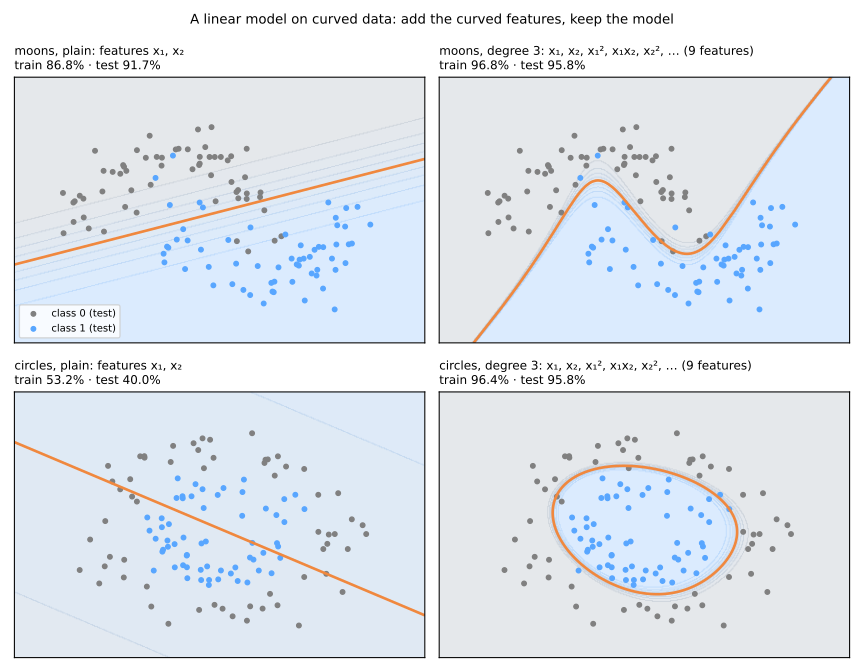
Moons: straight boundary 91.7%, degree 3 95.8%. Circles: straight line 40.0%, degree 3 95.8%

PolynomialFeatures(degree=3): 9 features; moons 0.917 → 0.958, circles 0.400 → 0.958.
On the circles, the 2 right features (100%) beat 9 generic ones: knowing the shape wins.
Prices: coefficients lose their reading, and more features overfit more. Scale after expanding.

Stage 3 · what if there are more than two classes?

Multi-class: softmax

\(k\) classes, one score per class, \(z_c = w_c^\top x + b_c\); the softmax turns them into probabilities that sum to 1:

\[ \hat{p}_c = \frac{e^{z_c}}{\sum_{j=1}^{k} e^{z_j}} \]

class	\(z_c\)	\(e^{z_c}\)	\(\hat p_c = e^{z_c}/11.212\)
A	2.0	7.389	0.659
B	1.0	2.718	0.242
C	0.1	1.105	0.099
sum		11.212	1.000

One weight vector and one intercept per class.
A gap of 1 in score is a factor \(e \approx 2.7\) in probability.
With two classes, softmax is the sigmoid: \(\sigma(z_1 - z_0)\).

On wine: a near tie

178 wines, 3 cultivars; two features, alcohol and flavanoids.

wine	true cultivar	scores	probabilities	predict
0	0	6.47, −0.22, −6.25	0.999, 0.001, 0	0
100	1	−0.29, 5.32, −5.02	0.004, 0.996, 0	1
133	2	−3.11, 1.56, 1.55	0.005, 0.502, 0.493	1 ✗

Wine 133 costs \(-\ln 0.493 \approx 0.706\), seven hundred times wine 0. Linear scores + softmax + cross-entropy is the output layer of essentially every neural classifier.

Stage 4 · when is logistic regression the right tool?

Practical profile

strengths

fast; convex: the same answer every time
reasonable probabilities
interpretable through odds ratios
a strong baseline

weaknesses

linear boundary
interactions added by hand
slow on unscaled features
correlated coefficients unstable to read

max_iter warnings usually mean unscaled features. One-hot columns for every category next to an intercept leave single coefficients meaningless: drop a reference category. Odds ratios are not probability ratios.

Summary

Squared error with a sigmoid caps the price of a mistake, kills the push on the worst ones and has plateaus; cross-entropy is convex.
The model is linear in its features: squared or polynomial features draw curved boundaries.
Knowing the shape beats generating many features; scale after expanding.
Softmax: one score per class, probabilities that sum to 1; with two classes it is the sigmoid.
Reach for it when you need a solid, explainable baseline with probabilities worth thresholding.

Advanced lab · about 25 min, in pairs

Odds ratios, and the one test, steps 7 and 8

Same notebook, same session: the steps use model, w, names, passengers, dummy and the train and test sets.
Read every coefficient as an odds ratio against its reference category; then touch the test set once, and move the threshold on the training rows.
Notebook on Colab (in Portuguese), from step 7.
Simulations: the odds ratio is the same for everyone (step 7) and moving the threshold (step 8).

Pace: step 7 and its simulation in 12 min; step 8 and its simulation in 10 min.