Machine Learning · Insper

Logistic Regression

A linear score, squashed into a probability

The first classifier of the course, and the neuron of every neural network

From numbers to categories

	classes	examples
binary	2, coded 0 and 1	pass/fail, fraud/legit, malignant/benign, survived/died
multiclass	\(k > 2\)	iris species, digit 0–9, product category

step 1: a probability

"this passenger survives with probability 0.94"

step 2: a threshold

"0.94 ≥ 0.5, so: survived"

Keep the two steps apart. You already own the pieces: the linear score and gradient descent. New: the sigmoid, cross-entropy and odds.

The path of this lesson

Why not a linea straight line fails at classifying
Score → probabilitysigmoid, decision boundary, odds
Loss & trainingcross-entropy, not squared error; gradient descent
Beyond the linecurved boundaries; many classes with softmax
Probability → labelthe threshold is a choice; when to use the model

Each stage answers one question: why can't a straight line classify? → how does a score become a probability we can read? → how do we measure the error and learn the weights? → what if the boundary curves, or there are more classes? → how does a probability become a decision?

Stage 1 · why can't a straight line classify?

Why not a straight line?

23 students, hours of study, pass (1) or fail (0). Fit a linear regression and call "pass" anything above 0.5.

Then add five students who studied 25 to 45 hours, and passed, as anyone would expect.

Predict. These five are easy, correctly labeled cases. Should they change where the line crosses 0.5?

Correct points hurt the line

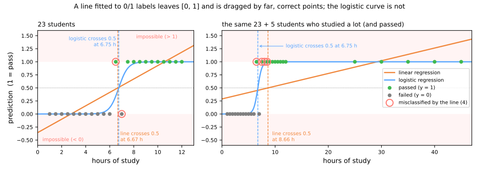
Left: on 23 students the line runs from −0.23 to 1.18 and crosses 0.5 at 6.67 h. Right: five far passers flatten the line, move its crossing to 8.66 h and double its errors; the logistic curve still crosses at 6.75 h

	line: outputs	line: crosses 0.5	line: errors	logistic: crosses 0.5	logistic: errors
23 students	−0.23 to 1.18	6.67 h	2	6.75 h	2
+ 5 far passers	0.31 to 1.39	8.66 h	4	6.75 h	2

Two problems, one cure

the line leaves [0, 1]

−0.23 for one hour, 1.18 for twelve: not probabilities, so "how sure is the model?" has no answer

correct points pull it

least squares wants the line near the far students: it flattens and the errors go from 2 to 4, caused by data that agreed with the model

A student with 45 hours sits on the flat part of the logistic curve, at probability ≈ 1: nothing left to correct, so it barely pulls. That flat part is the whole idea.

Stage 2 · how does a score become a probability we can read?

From line to probability

Keep the linear score:

\[ z = w^\top x + b \]

and squash it with the sigmoid:

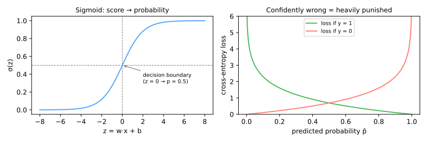
\[ \hat{p} = \sigma(z) = \frac{1}{1 + e^{-z}} \]

three values to memorize

\(\sigma(0) = 0.5\)
large positive \(z\) → \(\hat p \to 1\)
large negative \(z\) → \(\hat p \to 0\)

class 1 when \(\hat p \ge 0.5\), the same as \(z \ge 0\)

By hand: three new students

Fitted on the 23 students: \(w = 2.619\) per hour, \(b = -17.681\).

Predict. Before the table: who passes, the student with 4, 6 or 7.5 hours?

hours \(x\)	\(z = 2.619x - 17.681\)	\(e^{-z}\)	\(\hat p = 1/(1+e^{-z})\)	class
4	−7.205	1346	0.001	0 (fail)
6	−1.967	7.149	0.123	0 (fail)
7.5	1.962	0.1406	0.877	1 (pass)

A calculator is enough. In scikit-learn, predict_proba is literally sigmoid(decision_function).

The sigmoid, read in hours

The sigmoid with the three students: 4 h gets 0.001, 6 h gets 0.123, 7.5 h gets 0.877; the top axis shows the same curve in hours

The steepest point, \(\hat p = 0.5\), is at \(-b/w = 6.75\) hours. Less than two hours on either side go from "almost surely fails" to "almost surely passes". A larger \(w\) makes a sharper transition.

The decision boundary is a line

Two features: \(z = w_1x_1 + w_2x_2 + b\). Where \(z = 0\) (probability 0.5) is a straight line: a linear classifier.

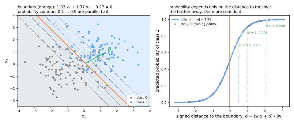
Left: the line 1.83·x₁ + 1.37·x₂ − 0.27 = 0 with parallel probability contours. Right: every point's probability on one curve σ(2.29·d) of its signed distance

200 points: \(w = (1.832, 1.371)\), \(b = -0.266\), \(\lVert w\rVert = 2.288\).

Probability depends only on the distance to the line

Walk away from the boundary along \(w\), from two different starting points of it:

signed distance \(d\)	−1	0	0.5	1	2
\(\hat p\), from either start	0.092	0.5	0.758	0.908	0.99

\[ \hat p = \sigma(\lVert w\rVert\, d) \]

\(w\) is perpendicular to the boundary and points toward class 1.
Equal-probability contours are lines parallel to the boundary.
\(\lVert w\rVert = 2.29\): one unit from the line, the model is already 90.8% sure.

Odds: the language of betting

probability \(p\)	odds \(p/(1-p)\)	in words
0.75	3	"3 to 1": out of 4 cases, 3 for and 1 against
0.5	1	"1 to 1": even
0.2	0.25	"1 to 4": out of 5 cases, 1 for and 4 against

\[ \frac{\hat p}{1 - \hat p} = e^{z} \qquad\Longleftrightarrow\qquad z = \ln \frac{\hat{p}}{1 - \hat{p}} = w^\top x + b \]

The score is the log of the odds, the logit. The model is linear in the log-odds, not in the probability.

One extra unit multiplies the odds

A model with \(w = 0.8\), \(b = -4\):

\(x\)	\(z = 0.8x - 4\)	\(\hat p = \sigma(z)\)	odds	\(e^{z}\)
4	−0.8	0.310	0.449	0.449
5	0.0	0.500	1.000	1.000
6	+0.8	0.690	2.226	2.226

\[ \frac{\text{odds}(x+1)}{\text{odds}(x)} = e^{w} = e^{0.8} = 2.226 \]

The honest sentence: one extra unit of \(x_j\) multiplies the odds by \(e^{w_j}\), everywhere on the curve, holding the other features fixed.

On the hours model

\(e^{w} = 13.727\)

hours	\(\hat p\)	odds
5	0.01	0.01
6	0.123	0.14
7	0.658	1.925

Each extra hour multiplies the odds of passing by 13.7.

In probability: +11 points from 5 to 6 hours, +54 points from 6 to 7.

The change in probability depends on where you start: largest near 0.5, vanishing in the tails. The odds ratio is the number doctors and credit analysts quote.

Stage 3 · how do we measure the error and learn the weights?

The loss: cross-entropy

Maximum likelihood: make the labels we observed as probable as possible. Take logs and flip the sign:

\[ J(w, b) = -\frac{1}{n} \sum_{i=1}^{n} \Big[ y_i \log \hat{p}_i + (1 - y_i) \log (1 - \hat{p}_i) \Big] \]

Only one term is alive per example: minus the log of the probability the model gave to the truth.

By hand: four predictions

Predict. Which of the four costs the most?

\(i\)	\(y\)	\(\hat p\)	probability given to the truth	\(-\ln(\cdot)\)
1	1	0.9	0.9	0.105
2	1	0.6	0.6	0.511
3	0	0.3	0.7	0.357
4	0	0.8	0.2	1.609

Mean: \((0.105 + 0.511 + 0.357 + 1.609)/4 = 0.646\). The confident mistake (point 4) is 62% of the total.

References: always saying 0.5 scores \(\ln 2 = 0.693\); a perfect model scores 0.

Each class has its curve

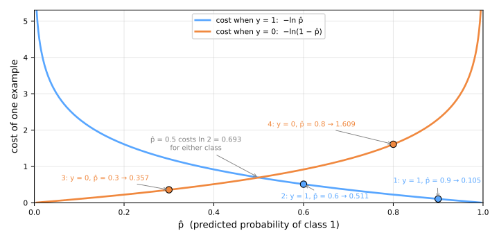
Two curves over p̂: −ln p̂ for class 1 and −ln(1 − p̂) for class 0, crossing at 0.5 with cost ln 2; the four examples of the table sit on them

Each curve is 0 at the correct end and grows without bound at the wrong end: from 0.8 to 0.99 for the wrong class, point 4 goes from 1.609 to 4.6.

Why not squared error?

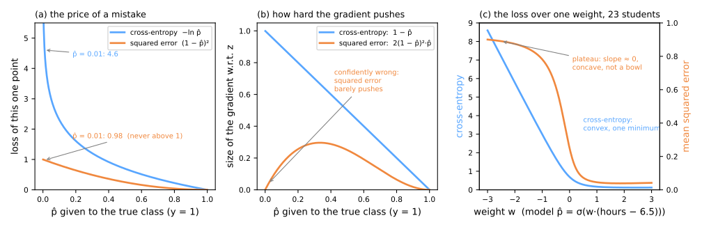
(a) cross-entropy grows without bound, squared error never exceeds 1; (b) cross-entropy pushes hardest on the worst mistakes; (c) cross-entropy is one convex valley, squared error has a plateau

(a) the price

squared error never exceeds 1: \(\hat p = 0.1\) and \(0.001\) cost 0.810 and 0.998

(b) the push

the worse the mistake, the weaker the squared-error gradient

(c) the shape

cross-entropy is convex; squared error has a plateau

(b) The push of the gradient

\[ \frac{\partial L}{\partial z} = \frac{\partial L}{\partial \hat p} \cdot \underbrace{\hat p\,(1 - \hat p)}_{\text{sigmoid slope}} \qquad \text{cross-entropy: } \frac{\partial L}{\partial z} = \hat p - y \]

\(\hat p\) given to the true class	sigmoid slope	squared error	cross-entropy
0.5	0.25	−0.250	−0.500
0.1	0.09	−0.162	−0.900
0.01	0.0099	−0.0196	−0.990
0.001	0.001	−0.0020	−0.999

With squared error the examples most in need of fixing are the ones it ignores (500 times weaker at 0.001). Cross-entropy's \(1/\hat p\) cancels the sigmoid's slope.

(c) The shape of the loss

One weight, \(\hat p = \sigma(w\,(\text{hours} - 6.5))\), on the 23 students. \(w < 0\) bets that whoever studies more fails.

\(w\)	−3	−1	0	+1	+3
squared error	0.900	0.782	0.250	0.045	0.042
cross-entropy	8.597	2.992	0.693	0.166	0.118

From \(w = -3\) squared error is a plateau (0.900 → 0.782); cross-entropy drops steeply (8.597 → 2.992). And it is convex: one valley, no local minima.

Simulator: the two losses side by side

Predict. Turn \(w\) the wrong way. Which loss notices that something is badly wrong?

Training by gradient descent

\[ \nabla_w J = \frac{1}{n} X^\top (\hat{p} - y), \qquad \frac{\partial J}{\partial b} = \frac{1}{n}\sum_i (\hat p_i - y_i) \]

The same shape as linear regression's gradient, with \(\hat p = \sigma(Xw + b)\) in place of \(Xw\).

forward: \(\hat p = \sigma(Xw + b)\)
loss: the cross-entropy \(J\)
backward: the gradients
update: \(w \leftarrow w - \eta\,\nabla_w J\)

iteration	loss
0	0.6931
10	0.3391
100	0.2956
1000	0.2955

The weights end within 0.0005 of scikit-learn's (1.8317, 1.3713): a convex function has only one bottom. The four names come back in neural networks.

Stage 4 · what if the boundary curves, or there are more classes?

Curved boundaries: engineer the features

The circles: one class inside, the other around it. Any line leaves pieces of the outer circle on both sides.

Predict. Give logistic regression \(x_1^2\) and \(x_2^2\) instead of \(x_1\) and \(x_2\). What shape can the boundary \(z = 0\) take now?

\[ z = w_1 x_1^2 + w_2 x_2^2 + b = 0 \quad\Longrightarrow\quad \text{with } w_1 \approx w_2 < 0, \text{ a circle} \]

features	test accuracy
\(x_1, x_2\)	0.400
\(x_1^2, x_2^2\)	1.000

\(w = (-16.83, -16.00)\), \(b = 9.70\): a circle of radius \(\approx 0.77\), between the inner circle (0.5) and the outer one (1).

When the shape is not obvious

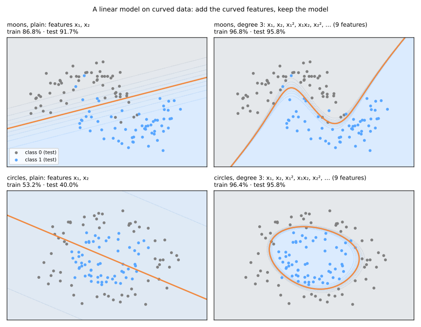
Moons: straight boundary 91.7%, degree 3 95.8%. Circles: straight line 40.0%, degree 3 95.8%

PolynomialFeatures(degree=3): 9 features; moons 0.917 → 0.958, circles 0.400 → 0.958.
On the circles, the 2 right features (100%) beat 9 generic ones: knowing the shape wins.
Prices: coefficients lose their reading, and more features overfit more. Scale after expanding.

Multi-class: softmax

\[ \hat{p}_c = \frac{e^{z_c}}{\sum_{j=1}^{k} e^{z_j}} \]

class	\(z_c\)	\(e^{z_c}\)	\(\hat p_c\)
A	2.0	7.389	0.659
B	1.0	2.718	0.242
C	0.1	1.105	0.099
sum		11.212	1.000

One weight vector and one intercept per class.
A gap of 1 in score is a factor \(e \approx 2.7\) in probability.
With two classes, softmax is the sigmoid.

On wine: a near tie

178 wines, 3 cultivars; two features, alcohol and flavanoids.

wine	true cultivar	scores	probabilities	predict
0	0	6.47, −0.22, −6.25	0.999, 0.001, 0	0
100	1	−0.29, 5.32, −5.02	0.004, 0.996, 0	1
133	2	−3.11, 1.56, 1.55	0.005, 0.502, 0.493	1 ✗

Wine 133 costs \(-\ln 0.493 \approx 0.706\), seven hundred times wine 0. Linear scores + softmax + cross-entropy is the output layer of essentially every neural classifier.

Stage 5 · how does a probability become a decision?

From probabilities to labels: the threshold

Predict. Lower the threshold from 0.5 to 0.2. What happens to the missed class-1 points, and to the false alarms?

threshold	class 1 predicted	missed class 1	false alarms	accuracy
0.2	131	1	32	0.835
0.5	97	12	9	0.895
0.8	76	31	7	0.810

0.5 is a choice, not part of the model. Accuracy counts both mistakes as equally bad; when a missed cancer is worse than a false alarm, move the threshold.

Practical profile

strengths

fast; convex: the same answer every time
reasonable probabilities
interpretable through odds ratios
a strong baseline

weaknesses

linear boundary
interactions added by hand
slow on unscaled features
correlated coefficients unstable to read

max_iter warnings usually mean unscaled features. Odds ratios are not probability ratios.

Summary

\(\hat p = \sigma(w^\top x + b)\): a linear score squashed into (0, 1); the boundary is a line.
\(e^{w_j}\) multiplies the odds per unit of \(x_j\).
Cross-entropy: minus the log of the probability given to the truth; convex.
Gradient \(\frac{1}{n}X^\top(\hat p - y)\): forward, loss, backward, update.
Curves need features; softmax for \(k\) classes; the threshold is a choice.

Lab · about 60 min, in pairs

Predicting survival on the Titanic

Open the notebook on Colab (in Portuguese) and save a copy to your Drive.
In each step, answer the Predict before running.
Simulations: the effect of age (step 5), one feature at a time (step 6), the odds ratio is the same for everyone (step 7), moving the threshold (step 8).
Compare with the output and the reading on the lesson page.

Pace: steps 1 to 4 in 20 min; steps 5 to 7 in 25 min; step 8 and the wrap-up in 15 min.