Machine Learning · Insper

The ML Landscape

Advanced approach

From a wish to a problem, why no model wins everywhere, and what goes wrong when a model's decisions reach people

The path of this part

Frame the problemtarget, moment, metric, baseline
No model wins everywherethe expected loss; no free lunch
Bias in the dataa model learns the past; proxies
Feedback loopsa model that decides what it will see

Each stage answers one question: what exactly is the problem? → why this model and not another? → what did the labels teach it? → does the model choose its own data?

Stage 1 · what exactly is the problem?

A wish is not a problem

"Reduce the number of patients who miss their appointments."

Predict. Before any data: what exactly would the model predict? When would it predict it, and what is known at that moment? How would you know it works?

Four questions before touching the data

question	what it fixes	the clinic
target	what is predicted, and so the task	missed the appointment: yes or no (classification)
moment	when, and so which features are allowed	48 h before: age, past absences, days since booking; not a cancellation call made the day before
metric	success, in the terms of whoever pays for errors	an empty slot vs one phone call: absences caught with the calls the staff can make
baseline	what the simplest answer scores	"nobody misses"; in regression, the training mean

A wrong moment is leakage: excellent in the lab, useless in production. Without a baseline, 0.80 means nothing. Sometimes the answer is a rule, not a model.

Stage 2 · why this model and not another?

The goal, written down

\[ \text{minimize } \underbrace{\mathbb{E}_{(x,y)\sim \mathcal{D}}\big[L\big(f(x),\,y\big)\big]}_{\text{expected loss on new data}} \quad \text{while only observing a finite sample} \]

\(f\): the model. \((x, y)\): a new example, drawn from \(\mathcal{D}\), the distribution of the data the model will meet (in the lab, the function draw).
\(L\): the loss, the price of one wrong answer (in the lab, the squared error \((y - f(x))^2\)). \(\mathbb{E}\): the average over all new examples.

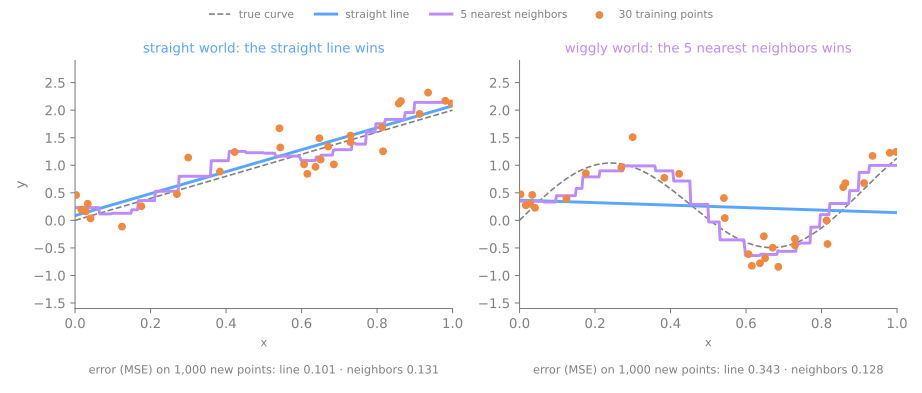
The lab's "new" column estimates it with 1,000 draws. With real data a test set does, if the model never saw it and \(\mathcal{D}\) does not drift.

No free lunch

Wolpert (1996): averaged over all possible problems, no learning algorithm is better than any other.
In practice: there is no universally best model. Try several families and validate.

Predict. Two worlds: a straight one (\(y = 2x\) plus noise) and a wiggly curve. Two models: a straight line, and 5 nearest neighbors (the average \(y\) of the 5 closest training points). Who wins where?

Two worlds, two winners

Straight world: the line wins, 0.101 against 0.131 for the neighbors. Wiggly world: the neighbors win, 0.128 against 0.343 for the line

30 training points, error on 1,000 new points. The line assumes a constant rate and wins where that is true; the neighbors assume only that close inputs have close answers. That set of assumptions is the model's inductive bias, and none wins everywhere.

What the theorem does not say

not: "all models are equal"

on your dataset some are much better; finding which is the job of validation and model selection

not: "experience is useless"

real problems are not drawn at random; some families (boosted trees on tables) win often, because their assumptions match

That is why the course teaches a portfolio: linear models, neighbors, kernels, trees, ensembles, networks, and always compares them on the same folds.

Stage 3 · what did the labels teach it?

Ethics: four questions before shipping a model

Models trained on historical data inherit historical bias.

fairness

equal performance across groups? A credit model trained on biased decisions reproduces them at scale

privacy

was the data collected with consent? can people be re-identified?

transparency

can decisions be explained to those affected?

feedback loops

does deploying the model change the data it will be retrained on? (predictive policing)

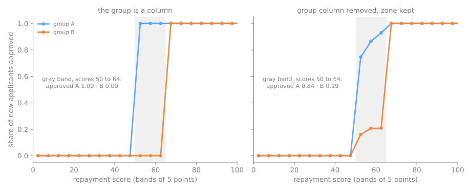
A model learns the past

4,000 past loans. Groups A and B repay alike, but officers approved A from a score of 50 and B only from 65. A small tree imitates them. Predict: at scores 50 to 64, what share of each group does it approve? And if the group column is deleted?

With the group as a column: in the 50 to 64 band, A approved 1.00, B 0.00. With the group removed and the zone kept: A 0.84, B 0.19

Left: the double standard, learned exactly. Right: the group is gone, but 80% of B live in one zone, and the zone carries the rule. A stand-in for a removed feature is a proxy: measure decisions by group, do not just delete columns.

Who owns the decision

"The model said so" is never an acceptable justification for a decision that affects people. You, the practitioner, own the consequences.

Stage 4 · does the model choose its own data?

A feedback loop, day by day

One patrol, two neighborhoods: A has 10 incidents a day, B has 12. The model sends the patrol where more crime is recorded; elsewhere only 2 calls a day get recorded. Predict: will the patrol ever go to B?

Why retraining does not fix it

Every record is a real incident; the records are wrong about where crime is, because the model decides where to look.
Each new model is trained on records the previous one shaped: after 30 days, A 355 against B 105.

explore

one day in five, send the patrol where it went less

measure per effort

incidents per patrolled day, not raw totals

Both together, in the lab: 9 days in A, 21 in B, and estimates of 10.0 and 12.0 a day, the truth. The same loop runs in recommender systems.

Summary: five questions for every project

Is the problem framed? Target, moment, metric, baseline, before the data.
What will the model meet? The expected loss on new data; a test set estimates it only if untouched.
Why this model? No free lunch: compare several families and validate.
What did the labels teach it? The past, biases included; proxies survive deleted columns.
Does it choose its own data? Then explore, and measure per unit of effort.

Next: Exploratory Data Analysis, the first contact with a dataset.

Advanced lab · about 30 min, in pairs

No free lunch, a biased past and a loop that feeds itself, steps 5 to 7

Step 5: two worlds, three models (the baseline among them), opposite winners.
Step 6: a tree trained on biased loan decisions, measured group by group.
Step 7: the patrol loop, run for 30 days.
Same Colab notebook as the fundamental lab, same session; at every step, the Predict first.
Simulations: delete the group column (step 6) and look where you do not look (step 7).

Pace: step 5 in 8 min; step 6 and the first simulation in 12 min; step 7 and the second in 10 min.