MLOps
A model in a notebook creates no value; predictions delivered reliably to the people who act on them do. Every lesson so far ended when the test score was printed. This one starts there. MLOps (machine-learning operations) is the set of engineering habits that take a fitted pipeline into production and keep it honest once it is there: packaging, serving, versioning, testing, monitoring and retraining. The workflow diagram of the first lessons promised that "deploy & monitor" loops back to the data; this lesson is that loop.
Each section below makes one idea concrete with a small measured experiment: what a model file really contains, what a pipeline does with a malformed request, how much a random seed changes, and how a statistic such as PSI detects that the world has moved. The lab at the end takes a real model through the whole loop, with real drift: a bank's telemarketing model is trained on calls from 2008–2009 and then meets the calls of 2009–2010, when the share of clients who said yes went from about 7% to more than 50%.
The loop drawn in the first section is the system; the lesson walks through it in five stages, drawn here: 1. package the model, what exactly goes into the file; 2. serve predictions, how requests reach the model and what it does with malformed ones; 3. reproduce and version, so that the running model can be rebuilt; 4. monitor drift, noticing that the world has changed; 5. ship changes safely, training–serving skew, feedback loops and replacing a model without breaking anything. Each stage links to its section, and in the slides a strip at the bottom shows which stage you are in.
- Package the modelthe whole pipeline, pickle risks, pinned versions, skops
- Serve predictionsbatch or online, schema checks, an endpoint, latency
- Reproduce and versionseeds, data fingerprints, an experiment log
- Monitor driftmeasuring a shift, late labels, retraining
- Ship changes safelytraining–serving skew, feedback loops, safe rollout, maturity
Slides
Click the slides and use the ← → arrows to navigate; F goes full screen and Esc shows every slide. Open the slides in a new tab
The model is the small box
Sculley et al. (2015), Hidden Technical Debt in Machine Learning Systems, made the observation that gave this field its agenda: in a production ML system, the code that learns is a small box surrounded by infrastructure (data collection, validation, feature extraction, serving, monitoring, configuration), and most failures happen in the infrastructure. This lesson's own lab illustrates the proportion: of its 212 lines of code (blank lines and comments not counted), 4 call fit and 5 more define the model. The rest load, check, package, serve, monitor and compare.
Every arrow is a place where something can break without raising an error:
| Stage | Fails silently when... | Section |
|---|---|---|
| Package | the file loads in another library version and predicts differently | Packaging |
| Serve | a malformed request still gets a confident-looking probability | Serving |
| Train again | nobody can say which data, code and seed produced the model in production | Reproducibility |
| Monitor | the world changes and the model keeps answering as if it had not | Monitoring |
| Serve vs train | the serving code computes a feature differently from the training code | Skew |
Packaging a model
The artifact is the whole pipeline
Stage 1. The pipelines lesson ended with one line, joblib.dump(pipe, ...). Here it is in context. The data is the German credit table (1,000 past loans; the target says whether the loan went bad), with three numeric columns and five categorical ones:
import os
import tempfile

import joblib
import numpy as np
import pandas as pd
from sklearn.compose import make_column_transformer
from sklearn.datasets import fetch_openml
from sklearn.linear_model import LogisticRegression
from sklearn.metrics import roc_auc_score
from sklearn.model_selection import train_test_split
from sklearn.pipeline import make_pipeline
from sklearn.preprocessing import OneHotEncoder, StandardScaler

credit = fetch_openml(data_id=31, as_frame=True)          # German credit: 1,000 past loans
num = ['duration', 'credit_amount', 'age']
cat = ['checking_status', 'savings_status', 'purpose', 'employment', 'housing']
X = credit.data[num + cat]
y = (credit.target == 'bad').astype(int)                  # 1 = the loan went bad
X_train, X_test, y_train, y_test = train_test_split(X, y, test_size=0.25, stratify=y,
                                                    random_state=0)

pipe = make_pipeline(
    make_column_transformer((StandardScaler(), num),
                            (OneHotEncoder(handle_unknown='ignore'), cat)),
    LogisticRegression(max_iter=1000))
pipe.fit(X_train, y_train)
proba = pipe.predict_proba(X_test)[:, 1]
print(f"test ROC AUC: {roc_auc_score(y_test, proba):.3f}")

folder = tempfile.mkdtemp()                               # a scratch folder for this lesson
path = os.path.join(folder, 'credit-pipeline.joblib')
joblib.dump(pipe, path)                                   # the WHOLE pipeline, one file
loaded = joblib.load(path)
print(f"{os.path.getsize(path):,} bytes on disk")
print("identical probabilities after reload:",
      np.array_equal(proba, loaded.predict_proba(X_test)[:, 1]))
The first check any packaging step must pass is the round trip: save, load, and compare the predictions bit for bit on the same rows. np.array_equal is the right test here, not "close enough": nothing in a save and load should change a single digit.
Why the whole pipeline and not just the model? Try to serve the model alone:
model_only = pipe[-1]                     # the LogisticRegression, without its preprocessing
try:
    model_only.predict_proba(X_test)
except ValueError as e:
    print('ValueError:', e)
print('the model expects', model_only.n_features_in_, 'columns; the raw table has', X_test.shape[1])
ValueError: X has 8 features, but LogisticRegression is expecting 30 features as input.
the model expects 30 columns; the raw table has 8
The logistic regression never saw the raw table. It saw the 30 columns produced by the column transformer: 3 standardized numbers and 27 one-hot indicators. A serving program that ships the model alone has to rebuild those 30 columns by hand, with the same means and standard deviations, the same category order and the same treatment of unknown values. Any difference produces wrong predictions without an error. Shipping the pipeline makes the preprocessing part of the artifact.
A pickle is a program
joblib files are Python pickles. A pickle is not a table of numbers; it is a sequence of instructions for rebuilding objects, and those instructions may include "call this function with these arguments". Any class can choose the function through __reduce__:
import pickle

class Innocent:
    def __reduce__(self):                 # tells pickle how to rebuild this object...
        return (print, ('this line ran while the file was being LOADED',))

blob = pickle.dumps(Innocent())
obj = pickle.loads(blob)                  # ...and loading obeys: it calls print(...)
Nothing was called explicitly; pickle.loads ran print because the file said so. Replace print with os.system and the file runs a shell command on the machine that loads it. The rule follows directly: load model files only from sources you would trust to run code on your machine, which for a model registry means controlling who can write to it.
Pin the versions
A pickle also records the version of the library that wrote it. scikit-learn stamps its version into every estimator it saves and compares the stamp when loading. To see what happens with a file from another version, we fake one by editing a single digit of the stamp:
import warnings

import sklearn
from sklearn.exceptions import InconsistentVersionWarning

raw = open(path, 'rb').read()
v = sklearn.__version__.encode()
print(f"the bytes {v!r} appear {raw.count(v)} time(s) inside the file")

# fake a file written by another version: same bytes, one digit of the stamp changed
fake = os.path.join(folder, 'old-pipeline.joblib')
open(fake, 'wb').write(raw.replace(v, b'0' + v[1:]))
with warnings.catch_warnings(record=True) as caught:
    warnings.simplefilter('always')
    joblib.load(fake)
stale = [w.message for w in caught if isinstance(w.message, InconsistentVersionWarning)]
print('InconsistentVersionWarning for:', list(dict.fromkeys(m.estimator_name for m in stale)))
print(str(stale[0])[:100] + '...')
the bytes b'1.9.0' appear 1 time(s) inside the file
InconsistentVersionWarning for: ['StandardScaler', 'OneHotEncoder', 'ColumnTransformer', 'LogisticRegression', 'Pipeline']
Trying to unpickle estimator StandardScaler from version 0.9.0 when using version 1.9.0. This might ...
Every estimator inside the pipeline complains, and the file still loads. That is the danger: the internal attributes of an estimator can change between versions, so a model may load and then predict differently, or fail later on a code path the test did not reach. The warning is easy to miss in a server log. Three habits handle it:
- store the versions (Python, scikit-learn, NumPy) next to the model, in a metadata file (the lab does this);
- pin them in the serving environment (
scikit-learn==1.9.0inrequirements.txt, or a container image); - when upgrading the library, retrain and re-validate rather than reload the old file. In a test suite,
warnings.simplefilter('error', InconsistentVersionWarning)turns the warning into a failure.
A safer format: skops
The skops library saves scikit-learn objects in a format that does not execute arbitrary code: on loading it rebuilds only types from an allow-list, and anything else must be trusted explicitly.
import skops.io as sio                    # pip install skops
from sklearn.preprocessing import FunctionTransformer

sk_path = os.path.join(folder, 'credit-pipeline.skops')
sio.dump(pipe, sk_path)
print('untrusted types in the plain pipeline:', sio.get_untrusted_types(file=sk_path))
same = np.array_equal(proba, sio.load(sk_path).predict_proba(X_test)[:, 1])
print('loaded without trusting anything, identical probabilities:', same)

def cap_amount(X):                        # a custom function inside the pipeline
    return np.minimum(X, 15000)

custom = make_pipeline(FunctionTransformer(cap_amount), LogisticRegression())
custom.fit(X_train[['credit_amount']], y_train)
custom_path = os.path.join(folder, 'custom.skops')
sio.dump(custom, custom_path)
print('untrusted types in the custom pipeline:', sio.get_untrusted_types(file=custom_path))
try:
    sio.load(custom_path)
except Exception as e:
    print('loading it without trust raises', type(e).__name__)
untrusted types in the plain pipeline: []
loaded without trusting anything, identical probabilities: True
untrusted types in the custom pipeline: ['__main__.cap_amount']
loading it without trust raises UntrustedTypesFoundException
The plain pipeline contains only scikit-learn and NumPy types, so it loads with no questions asked and predicts identically. The custom function cap_amount is code that skops does not know, so loading stops until someone reads the list and passes trusted=[...]. For serving outside Python, the ONNX format (through skl2onnx) converts a fitted pipeline into a portable graph that runtimes in C++, Java or JavaScript can execute.
Serving predictions
Batch, online, streaming, edge
Stage 2. How the model is called drives everything else in the architecture:
| Pattern | Latency | How the model is called | Example |
|---|---|---|---|
| Batch | hours | a scheduled job scores a whole table | nightly churn scores written to a database |
| Online (API) | milliseconds | one request, one answer, over HTTP | credit decision during checkout |
| Streaming | seconds | a consumer scores events from a queue | fraud flags on a transaction stream |
| Edge | on the device | the model ships inside an app | keyboard prediction on a phone |
Prefer batch whenever the decision can wait: it is cheaper (measured below), easier to monitor and easier to rerun. The rest of this section is about the online case, where a stranger's request reaches the model.
The pipeline accepts garbage
A pipeline checks very little. Five requests, one good and four broken in ways that happen in real systems:
good = {'duration': 24, 'credit_amount': 4000, 'age': 35, 'checking_status': '<0',
        'savings_status': '<100', 'purpose': 'new car', 'employment': '1<=X<4',
        'housing': 'own'}
requests = {
    'good request':        good,
    'age = -3':            {**good, 'age': -3},
    'amount in thousands': {**good, 'credit_amount': 4},
    'unseen purpose':      {**good, 'purpose': 'crypto'},
    'housing missing':     {k: v for k, v in good.items() if k != 'housing'},
}
for name, payload in requests.items():
    try:
        p = loaded.predict_proba(pd.DataFrame([payload]))[0, 1]
        print(f"{name:20s} P(bad) = {p:.3f}")
    except Exception as e:
        print(f"{name:20s} {type(e).__name__}: {str(e)[:45]}")
good request         P(bad) = 0.626
age = -3             P(bad) = 0.784
amount in thousands  P(bad) = 0.574
unseen purpose       P(bad) = 0.519
housing missing      ValueError: columns are missing: {'housing'}
Only the missing column raises an error. The other three broken requests get a probability that looks exactly as trustworthy as the good one. A negative age is standardized like any number. A loan of 4 Deutsche Mark is just a very small loan. The unknown purpose 'crypto' is encoded as all zeros by handle_unknown='ignore', which means "none of the purposes I know". With the default handle_unknown='error' it would have raised instead, so a new category appearing upstream would have taken the service down. Neither choice tells anyone that something is wrong.
A schema, and a function that checks it
The fix is to write down what the model saw in training, a schema, and check every request against it before predicting:
def make_schema(X):
    """What the model saw in training: a range per number, a list per category."""
    schema = {}
    for col in X.columns:
        if pd.api.types.is_numeric_dtype(X[col]):
            schema[col] = {'type': 'number', 'min': float(X[col].min()), 'max': float(X[col].max())}
        else:
            schema[col] = {'type': 'category', 'values': sorted(X[col].astype(str).unique())}
    return schema

def validate(payload, schema):
    """Return a list of problems; an empty list means the payload is acceptable."""
    errors = [f"unexpected field {k!r}" for k in payload if k not in schema]
    for col, rule in schema.items():
        v = payload.get(col)
        if v is None:
            errors.append(f"{col}: missing")
        elif rule['type'] == 'number':
            if isinstance(v, bool) or not isinstance(v, (int, float)):
                errors.append(f"{col}: expected a number, got {v!r}")
            elif not rule['min'] <= v <= rule['max']:
                errors.append(f"{col}: {v} outside training range [{rule['min']:g}, {rule['max']:g}]")
        elif v not in rule['values']:
            errors.append(f"{col}: unknown category {v!r}")
    return errors

schema = make_schema(X_train)
print(schema['age'])
print(schema['housing'])
{'type': 'number', 'min': 19.0, 'max': 75.0}
{'type': 'category', 'values': ['for free', 'own', 'rent']}
The serving function is then three lines of logic: validate, predict, and answer with the model version so that every logged answer can be traced back to the artifact that produced it.
def predict_one(payload, model=loaded, schema=schema, version='credit-2026.09.1'):
    """The whole serving contract: validate, predict, answer with the model version."""
    errors = validate(payload, schema)
    if errors:
        return {'status': 'rejected', 'errors': errors, 'model_version': version}
    p = float(model.predict_proba(pd.DataFrame([payload]))[0, 1])
    return {'status': 'ok', 'p_bad': round(p, 3), 'model_version': version}

for name, payload in requests.items():
    answer = predict_one(payload)
    print(f"{name:20s} {answer['status']:8s} {answer.get('p_bad', '')} {answer.get('errors', '')}")
good request         ok       0.626
age = -3             rejected  ['age: -3 outside training range [19, 75]']
amount in thousands  rejected  ['credit_amount: 4 outside training range [250, 15945]']
unseen purpose       rejected  ["purpose: unknown category 'crypto'"]
housing missing      rejected  ['housing: missing']
The good request gets the same 0.626 as before; each broken one is rejected with a message a human can act on. Whether "outside the training range" should reject or only warn is a business decision. A loan of 4 Deutsche Mark is certainly a unit bug, but a client older than anyone in the training data is a real person the model has simply never seen. The lab uses two levels, reject for impossible values and warn (predict, but log the warning) for values that are merely new. Libraries such as pydantic (built into FastAPI), pandera and Great Expectations express the same checks declaratively.
The same function behind an HTTP endpoint
The block below is not run on this page: FastAPI is a web framework, and a server does not belong inside a notebook. Save make_schema, validate and predict_one in a file service.py (loading the model with joblib.load), and this is the whole web service:
# app.py  (illustrative: run it from a terminal with uvicorn, not in a notebook)
from fastapi import FastAPI

from service import predict_one           # the tested function from this section

app = FastAPI()

@app.post('/predict')
def predict(payload: dict):
    return predict_one(payload)

@app.get('/health')                        # for the load balancer: "is the service alive?"
def health():
    return {'status': 'ok'}
$ pip install fastapi uvicorn
$ uvicorn app:app --port 8000
$ curl -X POST localhost:8000/predict -H 'Content-Type: application/json' \
       -d '{"duration": 24, "credit_amount": 4000, "age": 35, "checking_status": "<0",
            "savings_status": "<100", "purpose": "new car", "employment": "1<=X<4",
            "housing": "own"}'
{"status":"ok","p_bad":0.626,"model_version":"credit-2026.09.1"}
Notice where the logic lives. The web layer is a handful of lines with no decisions in them; everything that can be wrong is in predict_one, which is an ordinary function you can test in a notebook, as above. Production hardening adds a container (Docker) so that the pinned environment is the one that runs, a log of every request and answer (the raw material of monitoring), and a version in the URL (/v1/predict) so clients are not broken by the next model.
Latency: pay per call, not per row
How long does a prediction take? It depends much more on the number of calls than on the number of rows:
import time

def per_row_ms(model, rows, repeats=5):
    """Best of `repeats` timings, in milliseconds per row."""
    best = np.inf
    for _ in range(repeats):
        start = time.perf_counter()
        model.predict_proba(rows)
        best = min(best, time.perf_counter() - start)
    return 1000 * best / len(rows)

big = X_test.sample(10_000, replace=True, random_state=0)
one_at_a_time = np.mean([per_row_ms(loaded, big.iloc[[i]]) for i in range(200)])
in_one_batch = per_row_ms(loaded, big)
print(f"one row per call: {one_at_a_time:.3f} ms/row · 10,000 rows per call: {in_one_batch:.4f} ms/row"
      f" · ratio {one_at_a_time / in_one_batch:.0f}x")
Timings depend on the machine, so this block's output is not fixed. On the machine that built this page, one run printed:
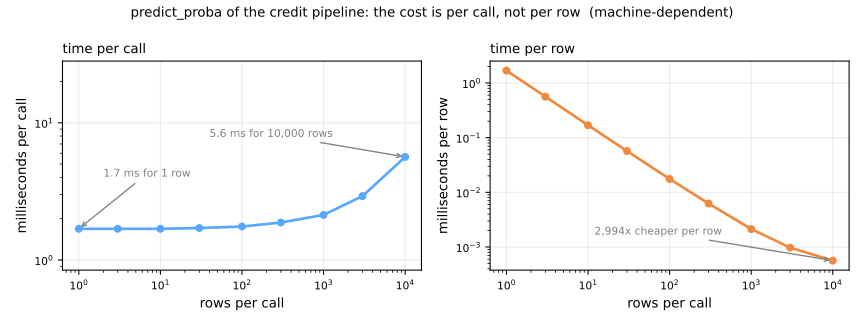
A call costs about 1.7 ms whether it carries one row or a thousand: that time goes into fixed work (building the DataFrame, checking column names, dispatching through three estimators), not into arithmetic. Scoring 10,000 rows in one call costs about 6 ms in total, between 2,500 and 3,000 times less per row than one call per row on this machine (the figure, which takes medians of several calls, lands near the top of that range). An HTTP request adds its own fixed cost (network, JSON parsing) on top. Two consequences: batch scoring is almost free, and an online service should keep the pipeline light, since the fixed overhead is paid on every request.
Reproducibility and versioning
Stage 3. "Which model is running, and could we rebuild it exactly?" can only be answered if every ingredient of the model has a version:
| Ingredient | What to record | Typical tool |
|---|---|---|
| Code | the commit that trained it | git |
| Data | a fingerprint (hash) and a way to get the same rows back | DVC, lakeFS, dated snapshots |
| Environment | library versions | requirements.txt, lock files, a container image |
| Randomness | every seed | random_state=... |
| Configuration | hyperparameters, features, thresholds | a config file under git |
| Results | validation metrics, the artifact itself | an experiment tracker, a model registry |
Seeds
Many estimators use randomness: a random forest draws bootstrap samples and random feature subsets. Two forests that differ only in their seed:
from sklearn.ensemble import RandomForestClassifier

def forest(seed):
    return make_pipeline(
        make_column_transformer((OneHotEncoder(handle_unknown='ignore'), cat),
                                remainder='passthrough'),
        RandomForestClassifier(n_estimators=200, random_state=seed)).fit(X_train, y_train)

p0, p1 = [forest(s).predict_proba(X_test)[:, 1] for s in (0, 1)]
p0_again = forest(0).predict_proba(X_test)[:, 1]
print(f"seed 0: AUC {roc_auc_score(y_test, p0):.3f} · seed 1: AUC {roc_auc_score(y_test, p1):.3f}")
print(f"seed 0 vs seed 1: {np.mean(p0 != p1):.0%} of probabilities differ, "
      f"{np.sum((p0 > 0.5) != (p1 > 0.5))} of {len(p0)} decisions flip")
print("seed 0 vs seed 0 again: identical =", np.array_equal(p0, p0_again))
seed 0: AUC 0.763 · seed 1: AUC 0.766
seed 0 vs seed 1: 96% of probabilities differ, 18 of 250 decisions flip
seed 0 vs seed 0 again: identical = True
The two AUCs are almost equal, so on the scoreboard the forests look like the same model. For the applicants they are not: 18 of the 250 test applicants (7%) get a different decision depending on the seed. Without random_state, every retraining draws a new seed, and a customer who asks "why was I refused yesterday and accepted today?" deserves a better answer than "we reran the script". With the seed fixed, the rerun is identical. Do not go the other way and try seeds until the test score is best: that is choosing on the test set, and the winner's curse applies.
Fingerprint the data
A model is a function of its training data, so the data needs an identity too. A hash of every row and value gives one:
import hashlib

def data_hash(df):
    """A fingerprint of the exact rows, values and order used for training."""
    row_hashes = pd.util.hash_pandas_object(df, index=True).to_numpy()
    return hashlib.sha256(row_hashes.tobytes()).hexdigest()[:12]

changed = X_train.copy()
changed.iloc[0, changed.columns.get_loc('age')] += 1          # one person one year older
print('training data    ', data_hash(X_train))
print('one value changed', data_hash(changed))
print('rows shuffled    ', data_hash(X_train.sample(frac=1, random_state=0)))
print('same data again  ', data_hash(X_train.copy()))
training data     68ad024c9661
one value changed 7eb64a1901f0
rows shuffled     a662547f0332
same data again   68ad024c9661
One changed value out of 6,000 gives a completely different fingerprint, and so does the same data in another order (order matters: cross-validation folds and some solvers depend on it). The same data gives the same fingerprint every time. Store it with the model; when someone asks whether a model was trained on this month's extract or last month's, the answer is a string comparison. A hash only identifies the data. To rebuild the model you also need the rows themselves, which is what data-versioning tools (DVC, lakeFS) or plain dated, read-only snapshots provide.
An experiment log
Put the ingredients together and each training run becomes one record. The simplest honest tracker is a file where each run appends one line and nothing is ever edited:
import json
import platform

from sklearn.model_selection import StratifiedKFold, cross_val_score

log_file = os.path.join(folder, 'runs.jsonl')

def log_run(params, metrics):
    """Append one experiment to a JSON-lines file: one line per run, never edited."""
    record = {'time': time.strftime('%Y-%m-%d %H:%M:%S'),
              'data': data_hash(X_train), 'python': platform.python_version(),
              'sklearn': sklearn.__version__, 'params': params, 'metrics': metrics}
    with open(log_file, 'a') as f:
        f.write(json.dumps(record) + '\n')

cv = StratifiedKFold(n_splits=5, shuffle=True, random_state=0)
for C in [0.01, 0.1, 1.0, 10.0]:
    candidate = pipe.set_params(logisticregression__C=C)
    auc = cross_val_score(candidate, X_train, y_train, cv=cv, scoring='roc_auc')
    log_run({'model': 'logistic', 'C': C}, {'cv_auc': round(auc.mean(), 4), 'cv_std': round(auc.std(), 4)})

runs = pd.json_normalize([json.loads(line) for line in open(log_file)])
print(runs[['data', 'params.C', 'metrics.cv_auc', 'metrics.cv_std']].to_string(index=False))
        data  params.C  metrics.cv_auc  metrics.cv_std
68ad024c9661      0.01          0.7495          0.0292
68ad024c9661      0.10          0.7599          0.0224
68ad024c9661      1.00          0.7522          0.0244
68ad024c9661     10.00          0.7442          0.0230
The log answers questions that memory cannot: which configurations were tried, on which data, with which library. C = 0.1 has the best mean (0.7599), but its lead over C = 1 (0.0077) is far below the fold standard deviations (about 0.02): without a fold-by-fold comparison, nothing says it is real, so treat the configurations as tied. Keep the losing runs too: they are the record of how many things were tried, which is exactly what the winner's curse depends on.
MLflow does the same with a web interface, artifact storage and a model registry that promotes versions from "staging" to "production". The block below is illustrative and not run here (MLflow is a large install):
import mlflow                                   # pip install mlflow

with mlflow.start_run():
    mlflow.log_params({'model': 'logistic', 'C': 0.1, 'data': data_hash(X_train)})
    mlflow.log_metric('cv_auc', 0.7599)
    mlflow.sklearn.log_model(pipe, name='model', registered_model_name='credit')
Monitoring and drift
Stage 4. Software usually breaks loudly; models decay silently. The service keeps answering 200 OK while its predictions get worse. Monitoring has three layers:
- System: latency, throughput, errors, the usual concerns of any web service;
- Data quality: schema violations, missing-value spikes, values outside the training range. Many incidents blamed on "the model" are upstream data incidents;
- Statistical drift: the world the model was trained on is no longer the world it is used in.
Three ways the world can change
A model is trained on a sample from a joint distribution \(P(x, y)\), and it can change in three basic ways. They are defined by what stays fixed (Moreno-Torres et al., 2012):
| Shift | What changes | What stays fixed | Example |
|---|---|---|---|
| Covariate shift (data drift) | \(P(x)\), the inputs | \(P(y \mid x)\) | the bank starts selling to younger clients |
| Concept drift | \(P(y \mid x)\), the relationship | \(P(x)\) | fraudsters change tactics; a crisis changes who repays |
| Prior shift (label shift) | \(P(y)\), the class balance | \(P(x \mid y)\) | an epidemic: more patients are sick, each one looks like before |
Before measuring what each one does to a model, we need a way to measure a change in a distribution. Two are standard.
Measuring a shift: PSI
The population stability index compares the share of rows that falls in each bin, with the bins cut on the reference (training) data:
where \(e_i\) is the expected share (reference) and \(a_i\) the actual share (current data) in bin \(i\). A worked example with 4 bins, cut at the quartiles of the training data, so each holds 25% of the reference rows:
| bin | \(e_i\) | \(a_i\) | \(a_i - e_i\) | \(\ln(a_i/e_i)\) | term |
|---|---|---|---|---|---|
| 1 | 0.25 | 0.10 | −0.15 | −0.916 | 0.1374 |
| 2 | 0.25 | 0.20 | −0.05 | −0.223 | 0.0112 |
| 3 | 0.25 | 0.30 | +0.05 | +0.182 | 0.0091 |
| 4 | 0.25 | 0.40 | +0.15 | +0.470 | 0.0705 |
| PSI | 0.228 |
Every term is positive, because \(a_i - e_i\) and \(\ln(a_i/e_i)\) always have the same sign. PSI is zero only when every bin keeps its share. (It is the Kullback–Leibler divergence taken in both directions, \(\text{KL}(a\|e) + \text{KL}(e\|a)\).) NumPy confirms the table:
e = np.array([0.25, 0.25, 0.25, 0.25])          # reference: the quartiles of the training data
a = np.array([0.10, 0.20, 0.30, 0.40])          # the share of this week's rows in each quartile
terms = (a - e) * np.log(a / e)
print(terms.round(4), '-> PSI =', terms.sum().round(3))
The usual reading, a convention from credit scoring (Siddiqi, 2006), is: below 0.1 no meaningful change, 0.1 to 0.25 a moderate change worth watching, above 0.25 a significant change. To give those numbers a meaning, here is PSI for a normal feature whose mean moves by a known amount, with 10 bins at the deciles of the reference:
def psi(ref, cur, bins=10, eps=1e-4):
    """Population stability index of `cur` against `ref`, on the reference's quantile bins."""
    edges = np.unique(np.quantile(ref, np.linspace(0, 1, bins + 1)))
    edges[0], edges[-1] = -np.inf, np.inf                    # open-ended outer bins
    e = np.histogram(ref, edges)[0] / len(ref)
    a = np.histogram(cur, edges)[0] / len(cur)
    e, a = np.clip(e, eps, None), np.clip(a, eps, None)      # an empty bin would give log(0)
    return float(np.sum((a - e) * np.log(a / e)))

rng = np.random.default_rng(0)
ref = rng.normal(0, 1, 5000)
for shift in [0.0, 0.1, 0.25, 0.5, 1.0]:
    print(f"mean moved by {shift:4.2f} sd -> PSI {psi(ref, rng.normal(shift, 1, 5000)):.3f}")
mean moved by 0.00 sd -> PSI 0.005
mean moved by 0.10 sd -> PSI 0.015
mean moved by 0.25 sd -> PSI 0.064
mean moved by 0.50 sd -> PSI 0.250
mean moved by 1.00 sd -> PSI 0.929
The alarm level 0.25 corresponds to the mean moving by half a standard deviation; one full standard deviation gives about 0.93. With no shift at all, PSI is not exactly zero (0.005): two samples of 5,000 rows never have identical histograms. The eps clip matters in practice: a bin that is empty in the current data would otherwise give \(\ln 0\).
Move the production distribution yourself. Find the shift where PSI crosses 0.25, then put the mean back at 0, change only the spread, and finally turn on concept drift:
With exact shares, half a standard deviation gives PSI 0.24; switch to 5,000-row samples (the setup of the code above) and sampling noise moves it a few hundredths either way, which is why the table shows 0.250. A wider or narrower spread with the same mean also moves PSI, through the outer bins. And concept drift, introduced in the table above and measured below, changes \(P(y \mid x)\) without moving a single row between bins: PSI stays at 0 while the accuracy falls.
Measuring a shift: the KS test
The Kolmogorov–Smirnov statistic compares the two empirical cumulative distribution functions and takes the largest vertical gap:
By hand, with five values on each side:
from scipy.stats import ks_2samp

ref_s, cur_s = np.array([1, 2, 3, 4, 5]), np.array([3, 4, 5, 6, 7])
grid = np.union1d(ref_s, cur_s)
F_ref = np.searchsorted(np.sort(ref_s), grid, side='right') / len(ref_s)
F_cur = np.searchsorted(np.sort(cur_s), grid, side='right') / len(cur_s)
print(pd.DataFrame({'x': grid, 'F_ref': F_ref, 'F_cur': F_cur, 'gap': np.abs(F_ref - F_cur)})
      .T.to_string(header=False))
res = ks_2samp(ref_s, cur_s)
print(f"by hand D = {np.abs(F_ref - F_cur).max():.1f} · scipy D = {res.statistic:.1f}, p-value = {res.pvalue:.3f}")
x      1.0  2.0  3.0  4.0  5.0  6.0  7.0
F_ref  0.2  0.4  0.6  0.8  1.0  1.0  1.0
F_cur  0.0  0.0  0.2  0.4  0.6  0.8  1.0
gap    0.2  0.4  0.4  0.4  0.4  0.2  0.0
by hand D = 0.4 · scipy D = 0.4, p-value = 0.873
At \(x = 2\), 40% of the reference is at or below it and none of the current sample is: \(D = 0.4\). The test then asks how surprising a gap of 0.4 would be if both samples came from the same distribution. With five points per side, not surprising at all: \(p = 0.873\). The figure shows both statistics on a larger example, 5,000 rows whose mean moved by half a standard deviation (figure script):
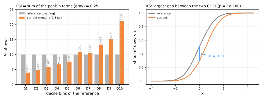
The two statistics answer different questions, and that matters with large data. A shift of 0.02 standard deviations is irrelevant for any model; watch what each statistic says about it as the number of rows grows:
rng = np.random.default_rng(1)
for n in [1_000, 10_000, 100_000, 1_000_000]:
    ref_n, cur_n = rng.normal(0, 1, n), rng.normal(0.02, 1, n)    # a shift of 0.02 sd
    print(f"n = {n:>9,}: KS p-value {ks_2samp(ref_n, cur_n).pvalue:.2g} · PSI {psi(ref_n, cur_n):.4f}")
n =     1,000: KS p-value 0.097 · PSI 0.0344
n =    10,000: KS p-value 0.14 · PSI 0.0018
n =   100,000: KS p-value 0.00049 · PSI 0.0004
n = 1,000,000: KS p-value 1.6e-41 · PSI 0.0005
The KS p-value answers "is there any difference?", and with enough rows the answer is always yes: at a million rows the same tiny shift gives \(p = 1.6 \times 10^{-41}\). PSI measures how large the difference is and stays near zero. At the other end, with 1,000 rows, PSI is noisier (0.034, almost all of it sampling noise). Two practical rules follow: with large batches, alert on magnitudes (PSI, or the KS statistic \(D\)) rather than on p-values; and when many features are tested at once, expect false alarms (50 features tested at the 5% level give about 2.5 alarms per batch with no drift at all), so correct the level (Bonferroni: divide it by the number of tests), as Rabanser et al. (2019) do in their benchmark of shift detectors.
The three shifts, measured
Now the three kinds of shift, simulated so that we know exactly which one happened. One feature \(x\); the probability of the positive class rises with \(x\), peaks at \(x = 1.5\) and falls again. The model is a small gradient-boosting classifier trained on \(x \sim N(0, 1)\). Each scenario draws 5,000 new rows:
from sklearn.ensemble import HistGradientBoostingClassifier

def true_p(x, move=0.0):
    """P(y = 1 | x): rises with x, peaks at x = 1.5 + move, then falls."""
    z = x - move
    return 1 / (1 + np.exp(-(3 * z - z ** 2)))

def draw(n, mean, rng, move=0.0):
    x = rng.normal(mean, 1, n)
    return x, (rng.random(n) < true_p(x, move)).astype(int)

rng = np.random.default_rng(2)
x_ref, y_ref = draw(5000, 0, rng)
model = HistGradientBoostingClassifier(max_depth=3, random_state=0).fit(x_ref.reshape(-1, 1), y_ref)

pool_x, pool_y = draw(100_000, 0, rng)                           # for the prior shift:
pos, neg = pool_x[pool_y == 1][:1000], pool_x[pool_y == 0][:4000]  # same P(x | y), 20% positives
scenarios = {'no change':       draw(5000, 0, rng),
             'covariate shift': draw(5000, 2.0, rng),            # P(x) moves, P(y | x) fixed
             'concept drift':   draw(5000, 0, rng, move=1.0),    # P(x) fixed, P(y | x) moves
             'prior shift':     (np.r_[pos, neg], np.r_[np.ones(1000), np.zeros(4000)].astype(int))}
rows = {}
for name, (x, y) in scenarios.items():
    p = model.predict_proba(x.reshape(-1, 1))[:, 1]
    rows[name] = {'PSI(x)': psi(x_ref, x), 'KS p': ks_2samp(x_ref, x).pvalue,
                  'accuracy': np.mean((p > 0.5) == y), 'precision': y[p > 0.5].mean(),
                  'actual rate': y.mean(), 'mean predicted': p.mean()}
print(pd.DataFrame(rows).T.round(3).to_string())
                 PSI(x)   KS p  accuracy  precision  actual rate  mean predicted
no change         0.004  0.695     0.816      0.769        0.462           0.465
covariate shift   3.505  0.000     0.728      0.729        0.720           0.780
concept drift     0.003  0.340     0.660      0.329        0.167           0.459
prior shift       0.152  0.000     0.794      0.491        0.200           0.339
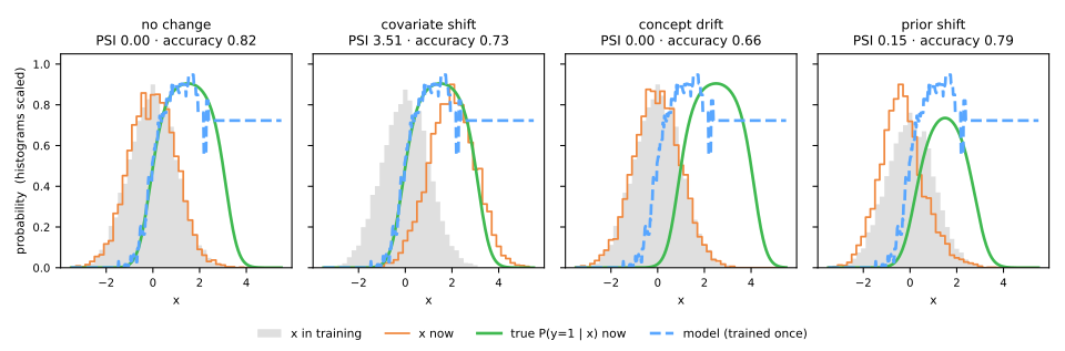
Read the table one row at a time:
- Covariate shift: the population moved to \(x \approx 2\), PSI 3.5, KS p-value zero; every input monitor fires. Accuracy falls because the model is now used where it had little data: past the peak, where the true probability turns down, the trees extend the last values they learned (the flat dashed blue curve on the right of the second panel).
- Concept drift: the inputs have not changed, PSI 0.003, KS p-value 0.34; no input monitor can see it. The same \(x\) now deserves a different answer, and the model's accuracy has fallen. Only the labels reveal concept drift.
- Prior shift: the positives went from 46% to 20%. The inputs move a little (PSI 0.15), accuracy barely changes, but precision drops and the probabilities are now too high: the model predicts 34% positives on average where 20% are positive. This is the effect of prevalence on precision, now happening in production.
Only concept drift is invisible without labels, but each shift breaks a different number, so a monitor needs both kinds of check: inputs (available at once) and outputs compared with outcomes (available later).
Labels arrive late
Ground truth is usually delayed: whether a customer churns is known after 60 days, whether a loan defaults after months or years. Monitoring therefore works in two speeds:
- immediately, on what the service sees: data-quality checks, PSI or KS of each input against the training reference, and the distribution of the model's own scores (the share flagged, the mean probability). Rabanser et al. (2019) found that testing the distribution of the model's outputs is one of the most effective shift detectors, and it costs one line;
- later, when outcomes arrive: the real metrics (AUC, precision, calibration), computed on each batch and compared with the validation estimate.
When labels come very late, or only for the cases the model approved (a refused loan never gets a repayment history), a small audited sample of labeled cases is the only protection against concept drift.
Degrade, detect, retrain
A drift that happens gradually is the common case in production. The same simulation, now as a year of monthly batches: the population moves 0.3 standard deviations per month. The static model is never touched. The monitored model is retrained on the month's labeled data whenever the PSI of its input, measured against the data it was trained on, crosses 0.25:
rng = np.random.default_rng(3)
new_model = lambda: HistGradientBoostingClassifier(max_depth=3, random_state=0)
static = new_model().fit(x_ref.reshape(-1, 1), y_ref)
live, live_ref = static, x_ref                 # the served model and its reference sample
print('month  mean   PSI  alert  static acc  live acc  best possible')
for month in range(13):
    x, y = draw(1000, 0.3 * month, rng)        # the population moves 0.3 sd per month
    X_m = x.reshape(-1, 1)
    drift = psi(live_ref, x)
    alert = drift > 0.25
    print(f"{month:5d} {0.3 * month:5.1f} {drift:5.2f}  {'ALERT' if alert else '     '} "
          f"{np.mean(static.predict(X_m) == y):10.3f} {np.mean(live.predict(X_m) == y):9.3f}"
          f" {np.mean((true_p(x) > 0.5) == y):14.3f}")
    if alert:                                  # the month's labels arrive: retrain on them
        live, live_ref = new_model().fit(X_m, y), x
month  mean   PSI  alert  static acc  live acc  best possible
    0   0.0  0.01             0.801     0.801          0.802
    1   0.3  0.09             0.809     0.809          0.815
    2   0.6  0.33  ALERT      0.780     0.780          0.785
    3   0.9  0.10             0.811     0.813          0.824
    4   1.2  0.33  ALERT      0.812     0.807          0.819
    5   1.5  0.14             0.783     0.805          0.814
    6   1.8  0.41  ALERT      0.759     0.814          0.830
    7   2.1  0.09             0.729     0.820          0.821
    8   2.4  0.30  ALERT      0.654     0.822          0.816
    9   2.7  0.18             0.507     0.807          0.805
   10   3.0  0.46  ALERT      0.417     0.803          0.802
   11   3.3  0.08             0.374     0.844          0.842
   12   3.6  0.34  ALERT      0.273     0.849          0.850
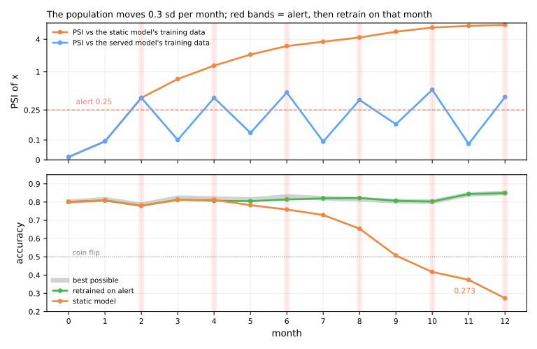
The static model degrades without a single error message: accuracy 0.801 in month 0, 0.654 in month 8, 0.273 in month 12. That is far worse than a coin flip, because the region the population moved into is one where the old answers are systematically inverted. The monitored model fires an alert every second month, retrains on that month's labels, and stays within about 0.02 of the best possible accuracy throughout.
Two details deserve attention. The first alert (month 2) fires when the static model is still fine (0.780, against a best possible of 0.785): drift is not damage. A PSI alert says the inputs changed, which is a reason to look and perhaps to retrain; it does not prove the model is broken. And retraining needed labels. Here they arrive at the end of each month; with a 60-day delay, the monitored model would always lag two months behind the drift.
Training–serving skew and other production failures
Skew, measured
Stage 5. Training–serving skew is any difference between how a feature is computed for training and how it is computed when serving. A classic cause is a new client application that sends a field in different units. The test set, three ways:
base = loaded.predict_proba(X_test)[:, 1]
skewed = {'as in training': X_test,
          'amount in thousands': X_test.assign(credit_amount=X_test['credit_amount'] / 1000),
          'duration in years': X_test.assign(duration=X_test['duration'] / 12)}
for name, data in skewed.items():
    p = loaded.predict_proba(data)[:, 1]
    rejected = np.mean([bool(validate(r, schema)) for r in data.to_dict('records')])
    print(f"{name:20s} AUC {roc_auc_score(y_test, p):.3f} · flagged {np.mean(p > 0.5):5.1%}"
          f" · decisions changed {np.mean((p > 0.5) != (base > 0.5)):5.1%} · rejected {rejected:4.0%}")
as in training       AUC 0.783 · flagged 20.0% · decisions changed  0.0% · rejected   1%
amount in thousands  AUC 0.775 · flagged 14.8% · decisions changed  5.2% · rejected 100%
duration in years    AUC 0.751 · flagged  2.8% · decisions changed 17.2% · rejected  93%
The AUC hardly moves (0.783 against 0.775 and 0.751), because the ranking is carried mostly by the other features. A dashboard that tracks AUC, if labels were even available, would see little. The decisions tell another story: with duration in years, 17.2% of the applicants get a different decision, and the share flagged as risky falls from 20.0% to 2.8%. The schema check catches both bugs at once, rejecting all rows in thousands and 93% of the rows in years. Even the untouched test set has 1% of rejections, because a few real applicants fall outside the training range, a reminder that rejection rules need the "reject or warn" decision discussed above.
Other common sources of skew:
- preprocessing reimplemented in the serving language (SQL, Java) instead of shipped inside the artifact;
- features computed from a batch table in training but from a live stream in serving ("average spend in the last 30 days" computed with different windows or time zones); feature stores such as Feast exist to compute each feature once for both paths;
- features that were available in the historical table but not at prediction time, the leakage of features that know the future. Offline the model looks excellent; in production the column does not exist yet. The lab measures one: the duration of a sales call, known only after the call has ended.
Feedback loops
Feedback loops
Once deployed, the model shapes the data it will be retrained on: the credit model only observes repayment for loans it approved; the recommender only sees clicks on items it showed. Naive retraining amplifies the model's own biases; recall the ethics lesson. Mitigations include holdout traffic (a small random share of decisions made without the model), careful sample weighting, and evaluating on data the model did not select.
Shipping a new model safely
A retrained model should replace the old one only after passing an evaluation gate: it must beat the current model on the same recent, labeled data that neither was trained on, by more than the noise (the paired comparison of the validation lesson). Then it is rolled out in stages:
| Strategy | How it works | What it protects against |
|---|---|---|
| Shadow | the new model scores live traffic, its answers are only logged | crashes, latency, strange score distributions, all with zero user impact |
| Canary | a small share of traffic (1–5%) is served by the new model | problems that only show with real users, limited to a few of them |
| A/B test | traffic is split at random and a business metric is compared | "better AUC" that does not translate into better outcomes |
| Rollback | the previous artifact stays in the registry, ready to serve | everything else: undoing must take minutes, not a retraining |
Tests and documentation
Breck et al. (2017), The ML Test Score, turned these ideas into a checklist of 28 tests in four groups: data, model development, infrastructure and monitoring. Examples, in paraphrase: feature expectations are captured in a schema; training is reproducible; training and serving compute the same feature values; the model is not too stale; prediction quality on served data has not regressed. Each test scores half a point if it is done manually and a full point if it is automated, and a system's score is the minimum over the four groups, since the weakest area is the one that causes the incident. Most of this lesson maps onto one of those tests: the round trip, the schema, the seeds, the data hash, the PSI checks.
The model itself needs documentation that travels with it. A model card (Mitchell et al., 2019) is a short document with fixed sections: model details, intended use, factors (groups and conditions the performance may depend on), metrics, evaluation data, training data, quantitative analyses, ethical considerations, and caveats and recommendations. The lab writes one from its own metadata and monitoring results.
Maturity, honestly
Most teams do not need a full platform on day one. A sensible ladder:
- notebook → script + versioned artifacts: a pipeline saved with its metadata, a data hash, an experiment log;
- manual deploy → CI/CD: tests (schema, round trip, a metric threshold on a fixed validation set) run automatically before any model ships;
- no visibility → logging + dashboards + drift alerts: every prediction logged with its model version, PSI and score distributions per batch;
- manual retraining → scheduled or triggered retraining with gates: a new model ships only if it beats the current one on recent data, with rollback ready.
Each rung eliminates one class of 3 a.m. incident. Climb when the pain justifies it: a model scored once a month for an internal report does not need a canary release.
The tool landscape
The ecosystem changes fast; the concepts above do not. A map, one line per tool, for when you need one:
| Job | Tools | In this lesson |
|---|---|---|
| Save a fitted model | joblib, skops, ONNX (skl2onnx) | joblib and skops |
| Serve over HTTP | FastAPI, BentoML | FastAPI sketch |
| Package the environment | Docker, requirements.txt, uv / conda lock files | pinned versions |
| Track experiments, register models | MLflow, Weights & Biases | a JSON-lines log |
| Version data | DVC, lakeFS | a data hash |
| Validate data | pandera, Great Expectations, pydantic | a schema function |
| Monitor drift | Evidently, NannyML, whylogs | PSI and KS by hand |
| Share features between training and serving | Feast | (skew section) |
| Schedule pipelines | Airflow, Prefect, Dagster | (retraining loop) |
Lab: shipping and monitoring a bank-marketing model
The setting is real. A Portuguese bank ran telemarketing campaigns for a term deposit between May 2008 and November 2010, and the UCI bank-marketing dataset records 45,211 of those calls in the order they were made: client attributes, contact history, and whether the client subscribed. We play the bank's data team: on 1 May 2009 a model trained on the previous year is deployed to rank clients before each call, and we follow it through the next 19 months. The drift that happens along the way is not simulated. It happened, during the financial crisis.
Steps 1–3 build and validate the model, steps 4–6 package it and put a guarded prediction function in front of it, steps 7–9 monitor it in production, step 10 retrains it and step 11 writes its model card. Files are written only to a temporary folder. Run the blocks in order, in one session; every output below is what the code prints (in a few seconds, once the data is downloaded). To work on it directly, download the lab notebook and open it in Jupyter or Colab (File → Upload notebook).
Step 1 — load the calls, in time order
import numpy as np
import pandas as pd
from sklearn.datasets import fetch_openml

raw = fetch_openml(data_id=1461, as_frame=True).frame        # UCI bank marketing, 45,211 calls
names = ['age', 'job', 'marital', 'education', 'default', 'balance', 'housing', 'loan',
         'contact', 'day', 'month', 'duration', 'campaign', 'pdays', 'previous', 'poutcome']
calls = raw.drop(columns='Class').set_axis(names, axis=1)
calls['y'] = (raw['Class'] == '2').astype(int)               # 1 = subscribed a term deposit

# the rows are in call order, May 2008 to November 2010, but the year is not stored:
# a new year starts each time a run of 'jan' calls begins
month = calls['month'].astype(str)
new_run = month.ne(month.shift())
year = 2008 + (new_run & month.eq('jan')).cumsum()
calls['date'] = pd.to_datetime(year.astype(str) + '-' + month, format='%Y-%b').dt.to_period('M')

print(calls.shape, calls['date'].min(), '->', calls['date'].max())
print(calls.groupby(calls['date'].dt.year)['y'].agg(['size', 'mean']).round(3))
The OpenML copy names the columns V1 to V16, so we restore the names from the dataset's documentation. The table has a month but no year; because the rows are in call order, a year can be rebuilt by counting the Januaries. Already the most important fact of the lab is visible: 5.1% of the 2008 calls ended in a subscription, 17.1% in 2009 and 51.6% in 2010, with far fewer calls. The bank changed who it called and how, in the middle of a crisis.
Step 2 — the column that will not exist when the model is used
from sklearn.compose import make_column_transformer
from sklearn.linear_model import LogisticRegression
from sklearn.metrics import roc_auc_score
from sklearn.pipeline import make_pipeline
from sklearn.preprocessing import OneHotEncoder, StandardScaler

CAT = ['job', 'marital', 'education', 'default', 'housing', 'loan', 'contact', 'poutcome']
NUM = ['age', 'balance', 'campaign', 'pdays', 'previous']
for c in CAT:
    calls[c] = calls[c].astype(str)

def make_model(num=NUM):
    return make_pipeline(
        make_column_transformer((OneHotEncoder(handle_unknown='ignore'), CAT),
                                (StandardScaler(), num)),
        LogisticRegression(max_iter=2000))

history = calls[calls['date'] < '2009-05']                 # the year before deployment
fit_part = history[history['date'] < '2009-02']            # May 2008 - Jan 2009
val_part = history[history['date'] >= '2009-02']           # Feb - Apr 2009, the most recent
for label, num in [('with duration', NUM + ['duration']), ('without duration', NUM)]:
    m = make_model(num).fit(fit_part[CAT + num], fit_part['y'])
    auc = roc_auc_score(val_part['y'], m.predict_proba(val_part[CAT + num])[:, 1])
    print(f"{label:17s} validation AUC {auc:.3f}")
Validation is temporal: fit on May 2008 – January 2009, validate on the three most recent months, as the validation lesson recommends for data with a time order. duration is the length of the sales call in seconds. It lifts the AUC from 0.619 to 0.757, and it is useless: the model must rank clients before the call, when the duration is not known. The dataset's own documentation warns about it, and the Gradient Boosting lab measured the same leak on a random split. This is the leakage of a feature that knows the future, and in production it would not fail with an error; the column would simply be missing, or filled with a default. We drop it, and also day and month, which record when the call happened rather than who the client is.
The honest AUC, 0.619, is modest. Predicting who will buy a deposit from a phone call's paperwork is hard, and we will not try to improve the model in this lab: the subject is what happens to it after deployment.
Step 3 — train the model the bank deploys in May 2009
from sklearn.metrics import brier_score_loss

FEATURES = CAT + NUM
m = make_model().fit(fit_part[FEATURES], fit_part['y'])
p_val = m.predict_proba(val_part[FEATURES])[:, 1]
validation = {'auc': round(float(roc_auc_score(val_part['y'], p_val)), 3),
              'brier': round(float(brier_score_loss(val_part['y'], p_val)), 3),
              'mean_predicted': round(float(p_val.mean()), 3),
              'actual_rate': round(float(val_part['y'].mean()), 3)}
print('validation (Feb-Apr 2009):', validation)

model = make_model().fit(history[FEATURES], history['y'])   # refit on the whole year
print(f"deployed model trained on {len(history):,} calls, {history['y'].mean():.1%} subscribed")
validation (Feb-Apr 2009): {'auc': 0.619, 'brier': 0.141, 'mean_predicted': 0.055, 'actual_rate': 0.158}
deployed model trained on 34,177 calls, 6.6% subscribed
The validation record has four numbers because they fail in different ways. The AUC (0.619) grades the ranking. The Brier score (0.141) and the comparison of the mean predicted probability with the actual rate grade the probabilities. And there the warning is already visible before deployment: in February–April 2009 the model predicted 5.5% subscriptions on average, while 15.8% subscribed. The world was already moving within the training year. The deployed model is refit on the whole year, 34,177 calls with 6.6% subscriptions.
Step 4 — package: the model, its metadata, a versioned folder
import hashlib
import json
import os
import platform
import tempfile

import joblib
import sklearn

def data_hash(df):
    return hashlib.sha256(pd.util.hash_pandas_object(df, index=True).to_numpy().tobytes()).hexdigest()[:12]

def make_schema(X, limits):
    """Training ranges and categories, plus hard limits that come from the business."""
    schema = {}
    for col in X.columns:
        if pd.api.types.is_numeric_dtype(X[col]):
            schema[col] = {'type': 'number', 'min': float(X[col].min()), 'max': float(X[col].max())}
            if col in limits:
                schema[col]['hard_min'], schema[col]['hard_max'] = limits[col]
        else:
            schema[col] = {'type': 'category', 'values': sorted(X[col].unique())}
    return schema

store = tempfile.mkdtemp()                                   # stands in for a model registry
version = 'bank-2009.05'
os.makedirs(os.path.join(store, version))
joblib.dump(model, os.path.join(store, version, 'model.joblib'))
metadata = {'version': version, 'trained_on': '2008-05 to 2009-04', 'rows': len(history),
            'data_hash': data_hash(history[FEATURES + ['y']]),
            'python': platform.python_version(), 'sklearn': sklearn.__version__,
            'features': FEATURES, 'schema': make_schema(history[FEATURES], {'age': (18, 100)}),
            'validation': validation}
with open(os.path.join(store, version, 'metadata.json'), 'w') as f:
    json.dump(metadata, f, indent=1)

print(sorted(os.listdir(os.path.join(store, version))))
print({k: metadata[k] for k in ['version', 'rows', 'data_hash', 'sklearn']})
print('pdays:', metadata['schema']['pdays'])
print('age:  ', metadata['schema']['age'])
['metadata.json', 'model.joblib']
{'version': 'bank-2009.05', 'rows': 34177, 'data_hash': 'b18de86a57b0', 'sklearn': '1.9.0'}
pdays: {'type': 'number', 'min': -1.0, 'max': 350.0}
age:   {'type': 'number', 'min': 19.0, 'max': 95.0, 'hard_min': 18, 'hard_max': 100}
The artifact is a folder named after the version, holding the pipeline and a JSON file with everything needed to trust it later: the training period and a hash of the training rows, the library versions, the list of features, the schema, and the validation metrics. The schema has two kinds of range. The training range comes from the data (pdays, the number of days since the client was last contacted, never exceeded 350 in the training year). The hard limits come from the business: a client is between 18 and 100 years old, whatever the data says. store stands in for a model registry; in a real system it would be MLflow, a bucket, or a shared folder that only the training job can write to.
Step 5 — reload and verify
import warnings

def load_artifact(folder):
    with open(os.path.join(folder, 'metadata.json')) as f:
        meta = json.load(f)
    if meta['sklearn'] != sklearn.__version__:
        warnings.warn(f"model built with scikit-learn {meta['sklearn']}, running {sklearn.__version__}")
    return joblib.load(os.path.join(folder, 'model.joblib')), meta

served, meta = load_artifact(os.path.join(store, version))
check = history[FEATURES].sample(2000, random_state=0)
same = np.array_equal(model.predict_proba(check), served.predict_proba(check))
print('reloaded model gives identical probabilities:', same)
print('data hash matches the metadata:', data_hash(history[FEATURES + ['y']]) == meta['data_hash'])
load_artifact is what the serving process runs at start-up. It checks the library version against the metadata before trusting the pickle, and the two prints are the tests that should run automatically before any deployment: the reloaded model reproduces the in-memory model exactly, and the data it claims to be trained on is the data we have.
Step 6 — a guarded predict function
def validate(payload, schema):
    """Errors reject the request; warnings let it through but are logged."""
    errors = [f"unexpected field {k!r}" for k in payload if k not in schema]
    warns = []
    for col, rule in schema.items():
        v = payload.get(col)
        if v is None:
            errors.append(f"{col}: missing")
        elif rule['type'] == 'category':
            if v not in rule['values']:
                errors.append(f"{col}: unknown category {v!r}")
        elif isinstance(v, bool) or not isinstance(v, (int, float)):
            errors.append(f"{col}: expected a number, got {v!r}")
        elif not rule.get('hard_min', -np.inf) <= v <= rule.get('hard_max', np.inf):
            errors.append(f"{col}: {v} is impossible")
        elif not rule['min'] <= v <= rule['max']:
            warns.append(f"{col}: {v} outside training range [{rule['min']:g}, {rule['max']:g}]")
    return errors, warns

def predict(payload, model=served, meta=meta):
    errors, warns = validate(payload, meta['schema'])
    if errors:
        return {'status': 'rejected', 'errors': errors, 'model_version': meta['version']}
    p = float(model.predict_proba(pd.DataFrame([payload])[meta['features']])[0, 1])
    return {'status': 'ok', 'p_subscribe': round(p, 3), 'warnings': warns,
            'model_version': meta['version']}

client = {'job': 'technician', 'marital': 'married', 'education': 'secondary', 'default': 'no',
          'housing': 'yes', 'loan': 'no', 'contact': 'cellular', 'poutcome': 'unknown',
          'age': 41, 'balance': 1200, 'campaign': 2, 'pdays': -1, 'previous': 0}
tests = {'good client': client,
         'missing balance': {k: v for k, v in client.items() if k != 'balance'},
         'age = 212': {**client, 'age': 212},
         'unseen job': {**client, 'job': 'influencer'},
         'age as text': {**client, 'age': '41'},
         'pdays = 400': {**client, 'pdays': 400, 'previous': 1, 'poutcome': 'failure'}}
for name, payload in tests.items():
    answer = predict(payload)
    detail = answer.get('errors') or answer.get('warnings') or ''
    print(f"{name:16s} {answer['status']:8s} {answer.get('p_subscribe', ''):<6} {detail}")
good client      ok       0.063
missing balance  rejected        ['balance: missing']
age = 212        rejected        ['age: 212 is impossible']
unseen job       rejected        ["job: unknown category 'influencer'"]
age as text      rejected        ["age: expected a number, got '41'"]
pdays = 400      ok       0.024  ['pdays: 400 outside training range [-1, 350]']
This is the function a web service would call (the FastAPI sketch in Serving wraps it unchanged). Six requests test its contract. The good client gets a probability. A missing field, an impossible age, an unknown job title and a number sent as text are rejected with a readable reason. The last client was contacted 400 days ago, longer than anyone in the training year, so the request is served with a warning. That is the right call here: as the next step shows, pdays values beyond 350 are not a bug, they are what time does to this feature.
Step 7 — production: monitors that need no labels
From May 2009 the model scores every call. Production is cut into calendar quarters; for each one we compute what is available immediately: how many requests the validator would reject or warn about, the PSI of every feature against the training year, and the PSI and KS statistic of the model's own score.
from scipy.stats import ks_2samp

def psi(ref, cur, bins=10, eps=1e-4):
    """PSI on quantile bins of `ref` (numbers) or on the categories (text)."""
    ref, cur = pd.Series(ref), pd.Series(cur)
    if pd.api.types.is_numeric_dtype(ref):
        edges = np.unique(np.quantile(ref, np.linspace(0, 1, bins + 1)))
        edges[0], edges[-1] = -np.inf, np.inf
        e = np.histogram(ref, edges)[0] / len(ref)
        a = np.histogram(cur, edges)[0] / len(cur)
    else:
        cats = sorted(set(ref) | set(cur))
        e = ref.value_counts(normalize=True).reindex(cats, fill_value=0).to_numpy()
        a = cur.value_counts(normalize=True).reindex(cats, fill_value=0).to_numpy()
    e, a = np.clip(e, eps, None), np.clip(a, eps, None)
    return float(np.sum((a - e) * np.log(a / e)))

production = calls[calls['date'] >= '2009-05'].copy()
production['batch'] = (production['date'].dt.qyear.astype(str) + 'Q'
                       + production['date'].dt.quarter.astype(str))
ref_score = served.predict_proba(history[FEATURES])[:, 1]

rows = []
for batch, g in production.groupby('batch'):
    checks = [validate(r, meta['schema']) for r in g[FEATURES].to_dict('records')]
    score = served.predict_proba(g[FEATURES])[:, 1]
    feature_psi = {c: psi(history[c], g[c]) for c in FEATURES}
    worst = max(feature_psi, key=feature_psi.get)
    rows.append({'batch': batch, 'calls': len(g),
                 'rejected': np.mean([bool(e) for e, w in checks]),
                 'warned': np.mean([bool(w) for e, w in checks]),
                 'worst feature': worst, 'its PSI': feature_psi[worst],
                 'score PSI': psi(ref_score, score),
                 'score KS D': ks_2samp(ref_score, score).statistic})
monitor = pd.DataFrame(rows).set_index('batch')
print(monitor.round(3))
        calls  rejected  warned worst feature  its PSI  score PSI  score KS D
batch
2009Q2   6217       0.0   0.147       contact    3.247      0.071       0.115
2009Q3   1261       0.0   0.053       contact    2.212      1.360       0.475
2009Q4    936       0.0   0.017       contact    2.112      1.390       0.446
2010Q1    799       0.0   0.041      poutcome    2.212      1.218       0.447
2010Q2    661       0.0   0.120      poutcome    2.145      0.891       0.391
2010Q3    865       0.0   0.148      poutcome    2.114      0.810       0.371
2010Q4    295       0.0   0.122      poutcome    2.295      1.098       0.439
How to read it, column by column:
- rejected is zero in every quarter: no missing fields, no unknown categories, no impossible values. The pipeline upstream is healthy;
- warned is not zero. In 2009Q2, 14.7% of the calls have a value outside the training range, almost all of them
pdaysabove 350. The training data began in May 2008, so nobody in it could have been contacted more than a year earlier; a year later, many clients have. The feature's range grows with time, and a hard rejection rule would have refused one call in seven; - worst feature is
contactin 2009, with a PSI above 2. In May and June 2008 the contact channel was not recorded (every value isunknown); from July 2008 it was. A change in how data is recorded looks exactly like drift, and a model trained on the 2008 mix partly learned "unknown channel" as a signal. From 2010 the worst feature ispoutcome, the outcome of the previous campaign: more and more clients had been called before, and many of them had said yes; - score PSI is small in 2009Q2 (0.071) and then jumps above 0.8 for every later quarter: the model's own output distribution moved, before any label arrived. This is the cheapest and most useful single monitor.
Step 8 — the labels arrive: how good was the model?
The outcome of a call is known within weeks, so by the end of each quarter the labels are in and the real metrics can be computed:
perf = []
for batch, g in production.groupby('batch'):
    score = served.predict_proba(g[FEATURES])[:, 1]
    perf.append({'batch': batch, 'actual rate': g['y'].mean(), 'mean predicted': score.mean(),
                 'AUC': roc_auc_score(g['y'], score), 'Brier': brier_score_loss(g['y'], score)})
perf = pd.DataFrame(perf).set_index('batch')
print(perf.round(3))
        actual rate  mean predicted    AUC  Brier
batch
2009Q2        0.124           0.081  0.671  0.105
2009Q3        0.367           0.150  0.584  0.276
2009Q4        0.459           0.158  0.609  0.326
2010Q1        0.517           0.174  0.664  0.347
2010Q2        0.551           0.167  0.698  0.372
2010Q3        0.519           0.157  0.710  0.350
2010Q4        0.427           0.174  0.749  0.271
The two kinds of metric tell different stories. The AUC stays between 0.584 and 0.749, never far from the validation value of 0.619 (and even above it later): the model still ranks clients about as well as it did. The probabilities collapse. The share of subscribers goes from 12.4% to above 50%, while the model keeps predicting around 16%, so in 2010Q2 it expects 16.7 subscriptions per 100 calls where 55.1 happen. The Brier score goes from 0.105 to 0.372. This is mostly prior shift, the base rate moving, plus the contact-history features changing meaning. A team that monitored only the AUC would conclude that nothing happened; a team that planned staff, budgets or call volumes from the predicted probabilities would be wrong by a factor of three.
Step 9 — alert rules
Monitors are only useful if someone is told when they fire. Rules are written down in advance, with thresholds; here, one per monitor:
alerts = pd.DataFrame({
    'rejections > 1%': monitor['rejected'] > 0.01,
    'warnings > 5%': monitor['warned'] > 0.05,
    'feature PSI > 0.25': monitor['its PSI'] > 0.25,
    'score PSI > 0.25': monitor['score PSI'] > 0.25,
    'calibration gap > 0.05': (perf['mean predicted'] - perf['actual rate']).abs() > 0.05,
    'AUC < validation - 0.05': perf['AUC'] < validation['auc'] - 0.05,
})
print(alerts.map(lambda fired: 'ALERT' if fired else '.').T.to_string())
batch                   2009Q2 2009Q3 2009Q4 2010Q1 2010Q2 2010Q3 2010Q4
rejections > 1%              .      .      .      .      .      .      .
warnings > 5%            ALERT  ALERT      .      .  ALERT  ALERT  ALERT
feature PSI > 0.25       ALERT  ALERT  ALERT  ALERT  ALERT  ALERT  ALERT
score PSI > 0.25             .  ALERT  ALERT  ALERT  ALERT  ALERT  ALERT
calibration gap > 0.05       .  ALERT  ALERT  ALERT  ALERT  ALERT  ALERT
AUC < validation - 0.05      .      .      .      .      .      .      .
Read it as a timeline. In the first production quarter, only the label-free data monitors fire: the out-of-range warnings (the growing pdays) and the feature PSI (the recording change in contact). The score distribution and the calibration are still acceptable, and a person looking at these alerts in mid-2009 would find two explainable changes rather than a broken model. From the second quarter on, the score PSI fires, and when the labels arrive the calibration gap confirms it. The AUC rule never fires. Choosing the metric to monitor is choosing what you are able to notice.
Step 10 — retrain on recent data, and compare
The fix for a moving base rate is to learn it again. A simple policy: at the start of each quarter, retrain the same pipeline on the last six months of labeled calls, and compare it on the quarter with the static model deployed in May 2009.
from sklearn.base import clone

compare = []
for batch, g in production.groupby('batch'):
    start = g['date'].min()
    recent = calls[(calls['date'] < start) & (calls['date'] >= start - 6)]   # last 6 labeled months
    retrained = clone(model).fit(recent[FEATURES], recent['y'])
    s_old = served.predict_proba(g[FEATURES])[:, 1]
    s_new = retrained.predict_proba(g[FEATURES])[:, 1]
    compare.append({'batch': batch, 'window': len(recent),
                    'AUC static': roc_auc_score(g['y'], s_old),
                    'AUC retrained': roc_auc_score(g['y'], s_new),
                    'Brier static': brier_score_loss(g['y'], s_old),
                    'Brier retrained': brier_score_loss(g['y'], s_new),
                    'gap static': s_old.mean() - g['y'].mean(),
                    'gap retrained': s_new.mean() - g['y'].mean()})
compare = pd.DataFrame(compare).set_index('batch')
print(compare.round(3).to_string())
print(compare.drop(columns='window').mean().round(3).to_string())
        window  AUC static  AUC retrained  Brier static  Brier retrained  gap static  gap retrained
batch
2009Q2   10059       0.671          0.682         0.105            0.103      -0.044         -0.035
2009Q3   12665       0.584          0.577         0.276            0.246      -0.218         -0.110
2009Q4   10196       0.609          0.619         0.326            0.253      -0.302         -0.135
2010Q1    2197       0.664          0.673         0.347            0.232      -0.343         -0.066
2010Q2    1735       0.698          0.673         0.372            0.227      -0.384         -0.050
2010Q3    1460       0.710          0.777         0.350            0.194      -0.362          0.002
2010Q4    1526       0.749          0.786         0.271            0.204      -0.253          0.132
AUC static         0.669
AUC retrained      0.684
Brier static       0.293
Brier retrained    0.208
gap static        -0.272
gap retrained     -0.037
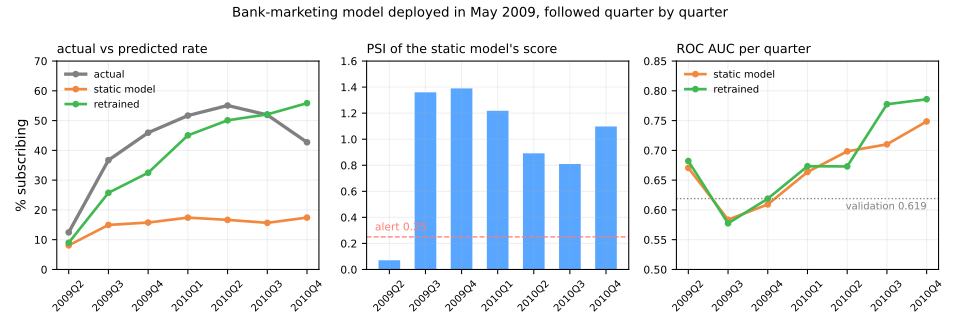
Retraining fixes what was broken. The calibration gap shrinks from −0.272 on average to −0.037, and the Brier score from 0.293 to 0.208. The ranking gains less, 0.684 against 0.669 on average and slightly worse in two quarters, with the largest gains at the end (0.777 against 0.710 in 2010Q3), when the retrained model has learned from clients whose previous campaign ended in a yes. The retrained model is not perfect either. It lags the rise in 2009Q3–Q4, because six months of history are still mostly the old world, and it overshoots in 2010Q4 (+0.132) when the rate falls back. Retraining on recent data is a bet that the recent past resembles the near future; the window length is the size of that bet.
In a real deployment each retrained model would pass the evaluation gate before replacing the current one, and each would be packaged as in step 4, with its own version folder and metadata.
Step 11 — a model card, generated from the metadata
worst_gap = (perf['mean predicted'] - perf['actual rate']).abs().idxmax()
card = f"""MODEL CARD - {meta['version']}
Model: logistic regression on {len(CAT)} categorical and {len(NUM)} numeric client features, scikit-learn {meta['sklearn']}
Intended use: rank clients before a term-deposit call. Not for credit or pricing decisions.
Training data: {meta['rows']:,} calls, {meta['trained_on']}, hash {meta['data_hash']}
Excluded: duration (known only after the call), day and month (calendar, not client)
Validation, Feb-Apr 2009: AUC {meta['validation']['auc']}, Brier {meta['validation']['brier']}, \
predicted rate {meta['validation']['mean_predicted']:.1%} vs actual {meta['validation']['actual_rate']:.1%}
Production, {perf.index[0]} to {perf.index[-1]}: AUC {perf['AUC'].min():.2f} to {perf['AUC'].max():.2f}; \
worst calibration in {worst_gap}: predicted {perf.loc[worst_gap, 'mean predicted']:.1%}, actual {perf.loc[worst_gap, 'actual rate']:.1%}
Caveats: pdays grows past its training range over time; contact was not recorded before July 2008;
probabilities are not calibrated after a change in the base rate. Retrain quarterly on the last 6 months.
"""
print(card)
MODEL CARD - bank-2009.05
Model: logistic regression on 8 categorical and 5 numeric client features, scikit-learn 1.9.0
Intended use: rank clients before a term-deposit call. Not for credit or pricing decisions.
Training data: 34,177 calls, 2008-05 to 2009-04, hash b18de86a57b0
Excluded: duration (known only after the call), day and month (calendar, not client)
Validation, Feb-Apr 2009: AUC 0.619, Brier 0.141, predicted rate 5.5% vs actual 15.8%
Production, 2009Q2 to 2010Q4: AUC 0.58 to 0.75; worst calibration in 2010Q2: predicted 16.7%, actual 55.1%
Caveats: pdays grows past its training range over time; contact was not recorded before July 2008;
probabilities are not calibrated after a change in the base rate. Retrain quarterly on the last 6 months.
A model card is short on purpose: it is the page someone reads before using the model for something new. Every number in this one is computed from the metadata of step 4 and the monitoring of step 8, so the card can be regenerated with each version instead of drifting out of date in a wiki. The "intended use" line is the one that prevents the most damage. A ranking model for telemarketing, with probabilities off by a factor of three, must not be reused to price a loan.
Your turn
- Serve it. Save
load_artifact,validateandpredictin a fileservice.py(loading the artifact at import time), adapt the FastAPI sketch from the Serving section intoapp.py, and runuvicorn app:app. Send the good client withcurl, then the client with"age": "41". What HTTP status code does the rejection come back with, and should it be 200? - Break the pipe. In the 2010Q1 batch only, divide
balanceby 1,000 (an upstream unit change) and rerun steps 7–9. Which monitors fire? Does the AUC notice? Does the rejection rate? - The window. Rerun step 10 with windows of 3 and 12 months, and with all the history up to each quarter. Which window gives the best mean Brier score, and which the best mean AUC? Why is "all history" bad for calibration here?
- Many tests at once. For the first production quarter, run
ks_2sampon each of the 5 numeric features and count how many have \(p < 0.05\). Then apply a Bonferroni correction (\(p < 0.05/5\)). Repeat on two random halves of the training year, where no drift is expected. What does that say about alerting on p-values with thousands of rows?
Class materials
Lab notebook
The lab above as a notebook, ready for Jupyter or Colab: lab-mlops.ipynb.
Further reading
- scikit-learn User Guide — Model persistence: pickle, joblib, skops and ONNX compared, with the security caveats
- FastAPI tutorial
- MLflow documentation: tracking and model registry
- Evidently documentation: drift reports built on the statistics of this lesson
- Huyen, C. Designing Machine Learning Systems. O'Reilly (2022): data distribution shifts, monitoring and continual learning, at book length
References
- Sculley, D.; Holt, G.; Golovin, D.; Davydov, E.; Phillips, T.; Ebner, D.; Chaudhary, V.; Young, M.; Crespo, J.-F.; Dennison, D. "Hidden Technical Debt in Machine Learning Systems." Advances in Neural Information Processing Systems 28 (NeurIPS 2015): 2503–2511 — the ML code as a small box inside a large system. full text
- Breck, E.; Cai, S.; Nielsen, E.; Salib, M.; Sculley, D. "The ML Test Score: A Rubric for ML Production Readiness and Technical Debt Reduction." IEEE International Conference on Big Data (2017): 1123–1132 — 28 tests in four groups. DOI
- Mitchell, M.; Wu, S.; Zaldivar, A.; Barnes, P.; Vasserman, L.; Hutchinson, B.; Spitzer, E.; Raji, I. D.; Gebru, T. "Model Cards for Model Reporting." Proceedings of the Conference on Fairness, Accountability, and Transparency (FAT* 2019): 220–229. DOI
- Rabanser, S.; Günnemann, S.; Lipton, Z. C. "Failing Loudly: An Empirical Study of Methods for Detecting Dataset Shift." Advances in Neural Information Processing Systems 32 (NeurIPS 2019) — two-sample tests on features and on model outputs, compared. arXiv
- Moreno-Torres, J. G.; Raeder, T.; Alaiz-Rodríguez, R.; Chawla, N. V.; Herrera, F. "A Unifying View on Dataset Shift in Classification." Pattern Recognition 45, no. 1 (2012): 521–530 — covariate shift, prior probability shift and concept shift, defined. DOI
- Gama, J.; Žliobaitė, I.; Bifet, A.; Pechenizkiy, M.; Bouchachia, A. "A Survey on Concept Drift Adaptation." ACM Computing Surveys 46, no. 4 (2014): 44. DOI
- Siddiqi, N. Credit Risk Scorecards: Developing and Implementing Intelligent Credit Scoring. Wiley (2006) — the population stability index and its usual thresholds.
- Moro, S.; Cortez, P.; Rita, P. "A Data-Driven Approach to Predict the Success of Bank Telemarketing." Decision Support Systems 62 (2014): 22–31 — the bank-marketing data used in the lab (UCI, OpenML 1461). DOI