Machine Learning · Insper

MLOps

Advanced approach

What breaks in production that no test set shows, and how to replace a running model safely

The path of this part

Package and serve at scaleskops and ONNX, latency per call
Track every runan experiment log, a model registry
Detect and reactp-values with big data; degrade, detect, retrain
Ship changes safelyskew, feedback loops, gated rollout, tests, maturity

Each stage answers one question: what changes when the model leaves the notebook? → why was this model chosen, among all those tried? → which alarm is real, and when should we retrain? → what else breaks, and how do we replace a model safely?

Stage 1 · what changes when the model leaves the notebook?

A safer format: skops

A joblib file is a pickle, so loading it can run code. On loading, skops rebuilds only types from an allow-list; anything else must be trusted explicitly.

pipeline	untrusted types	loading without trust
scaler + one-hot + logistic	`[]`	loads, identical probabilities
with a custom function	`['__main__.cap_amount']`	`UntrustedTypesFoundException`

Outside Python, ONNX (Open Neural Network Exchange, through skl2onnx) turns a fitted pipeline into a portable graph for C++, Java or JavaScript runtimes.

Latency: pay per call, not per row

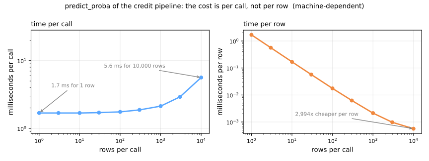
Predict. Scoring one row per call, or 10,000 rows in one call: how different is the cost per row?

Time per call is flat at about 1.7 ms from 1 to about 1,000 rows, then grows; the cost per row falls from 1.7 ms to 0.0006 ms

On the machine that built the page: 1.724 ms/row one at a time, 0.0006 ms/row in one batch, about 2,700×. A call costs about 1.7 ms whether it carries one row or a thousand: fixed work, not arithmetic.

Stage 2 · why was this model chosen, among all those tried?

An experiment log: one line per run, never edited

data	C	CV AUC	CV std
68ad024c9661	0.01	0.7495	0.0292
68ad024c9661	0.10	0.7599	0.0224
68ad024c9661	1.00	0.7522	0.0244
68ad024c9661	10.00	0.7442	0.0230

CV: cross-validation; std: standard deviation across the folds; AUC: area under the ROC curve; C: the inverse of the logistic regression's penalty.

The lead of C = 0.1 over C = 1 (0.0077) is far below the fold standard deviations (about 0.02): treat them as tied. Keep the losing runs: they record how many things were tried. MLflow does the same with a web interface and a model registry.

Stage 3 · which alarm is real, and when should we retrain?

p-values with big data

Predict. A feature's mean moves by 0.02 standard deviations (sd), an irrelevant shift. As the batch grows from 1,000 to a million rows, what happens to the KS (Kolmogorov–Smirnov) p-value? And to PSI?

a shift of 0.02 sd, n =	1,000	10,000	100,000	1,000,000
KS p-value	0.097	0.14	0.00049	1.6e-41
PSI (population stability index)	0.0344	0.0018	0.0004	0.0005

The p-value answers "is there any difference?": with enough rows, always yes. Alert on magnitudes (PSI, or the KS statistic \(D\)). With many features, correct for multiple tests: 50 features at the 5% level give about 2.5 false alarms per batch.

Degrade, detect, retrain

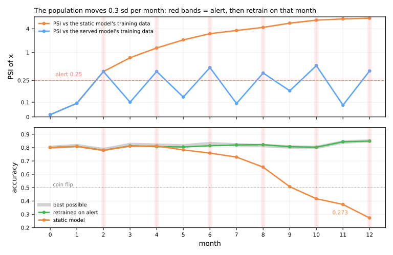
The population moves 0.3 sd per month. Static model vs a model retrained whenever its input PSI crosses 0.25.

month	static	monitored	best possible
0	0.801	0.801	0.802
2 (alert)	0.780	0.780	0.785
6	0.759	0.814	0.830
8	0.654	0.822	0.816
12	0.273	0.849	0.850

PSI of the input grows past 4 for the static model; static accuracy falls from 0.80 to 0.27 while the retrained model tracks the best possible

The first alert fires while the static model is still fine: drift is not damage. And retraining needs labels: with a 60-day delay, the monitored model lags two months.

Stage 4 · what else breaks, and how do we replace a model safely?

Training–serving skew, measured

A new client application sends a field in different units. The test set, three ways:

	AUC	flagged	decisions changed	rejected by the schema
as in training	0.783	20.0%	0.0%	1%
amount in thousands	0.775	14.8%	5.2%	100%
duration in years	0.751	2.8%	17.2%	93%

The AUC hardly moves; the decisions do. The schema catches both bugs. Other sources: preprocessing reimplemented in SQL (Structured Query Language) or Java, different time windows, features that know the future.

Shipping a new model safely

First an evaluation gate: beat the current model on recent labeled data neither saw, by more than the noise. Then roll out in stages:

strategy	how	protects against
shadow	scores live traffic, answers only logged	crashes, latency, strange scores
canary	1–5% of traffic	problems that only show with real users
A/B test	random split, a business metric	"better AUC" that is not better outcomes
rollback	the previous artifact stays ready	everything else, in minutes

Feedback loops: the credit model only sees repayment for loans it approved. Keep holdout traffic decided without the model.

Tests, documentation, and maturity

The ML Test Score

28 tests in 4 groups: data, model development, infrastructure, monitoring (Breck et al., 2017). The score is the minimum over the groups.

Model card

intended use, factors, metrics, training and evaluation data, ethical considerations, caveats (Mitchell et al., 2019)

A sensible ladder

script + versioned artifacts
CI/CD (continuous integration and delivery): tests before any model ships
logging, dashboards, drift alerts
retraining with gates and rollback

Climb when the pain justifies it.

The tool landscape

job	tools	in this lesson
save a fitted model	joblib, skops, ONNX	joblib and skops
serve over HTTP	FastAPI, BentoML	FastAPI sketch
package the environment	Docker, lock files	pinned versions
track experiments, register models	MLflow, Weights & Biases	a JSON-lines log
version data	DVC (Data Version Control), lakeFS	a data hash
validate data	pandera, Great Expectations, pydantic	a schema function
monitor drift	Evidently, NannyML, whylogs	PSI and KS by hand

HTTP: the web's protocol; JSON-lines: one JSON record per line. The ecosystem changes fast; the concepts do not.

Summary

A pickle runs code; skops loads only trusted types. A call costs a fixed time: batch when you can.
Log every run, losers included; ties within the fold noise are ties.
With big batches, alert on magnitudes, not p-values; drift is not damage, and retraining needs labels.
Skew changes decisions while the AUC barely moves; the schema catches it.
New models pass a gate and roll out in stages, with rollback ready.

Advanced lab · about 30 min, in pairs

Alerts, retraining and a model card, steps 9 to 11

Same notebook, same session: the steps use production, served, meta, monitor and perf from steps 1 to 8.
Turn the monitors into alert rules, retrain every quarter on the last six months, generate the model card from the metadata.
Lab notebook, from step 9. Answer the Predict before running.
Simulations: monthly batches (step 9) and fix only the base rate (step 10).

Pace: step 9 and its simulation in 12 min; step 10 and its simulation in 13 min; step 11 in 5 min.