This lesson starts where the others ended
- Every lesson so far ended when the test score was printed.
- Value comes from predictions delivered reliably to the people who act on them.
- MLOps (machine-learning operations): the engineering habits that take a fitted pipeline into production and keep it honest there.
The model is the small box
Sculley et al. (2015), Hidden Technical Debt in Machine Learning Systems: the code that learns is a small box surrounded by infrastructure, and most failures happen in the infrastructure.
fit + define the modelThe rest load, check, package, serve, monitor and compare.
The loop, and what the monitor sends back
Click the buttons: what does a drift alert send back, and what does a data bug?
Every arrow can break without an error
| stage | fails silently when... |
|---|---|
| package | the file loads in another library version and predicts differently |
| serve | a malformed request still gets a confident-looking probability |
| train again | nobody can say which data, code and seed produced the model in production |
| monitor | the world changes and the model keeps answering as if it had not |
| serve vs train | the serving code computes a feature differently from the training code |
The path of this lesson
- Package the modelthe whole pipeline, pickle risks, pinned versions, skops
- Serve predictionsbatch or online, schema checks, an endpoint, latency
- Reproduce and versionseeds, data fingerprints, an experiment log
- Monitor driftmeasuring a shift, late labels, retraining
- Ship changes safelytraining–serving skew, feedback loops, safe rollout, maturity
Packaging: the artifact is the whole pipeline
German credit (1,000 past loans): 3 numeric and 5 categorical columns → scaler + one-hot → logistic regression.
joblib.dump(pipe, path)                  # the WHOLE pipeline, one file
loaded = joblib.load(path)
np.array_equal(proba, loaded.predict_proba(X_test)[:, 1])
test ROC AUC
on disk
round trip
Why not ship the model alone?
LogisticRegression out of the pipeline and give it the raw table. What happens?
ValueError: X has 8 features, but LogisticRegression is expecting 30 features as input.
- The model saw the 30 columns of the column transformer: 3 standardized numbers + 27 one-hot indicators.
- Serving it alone means rebuilding those 30 columns by hand: same means, same category order, same unknowns. Any difference gives wrong predictions without an error.
A pickle is a program
class Innocent:
    def __reduce__(self):                 # tells pickle how to rebuild this object...
        return (print, ('this line ran while the file was being LOADED',))

obj = pickle.loads(pickle.dumps(Innocent()))   # ...and loading obeys
this line ran while the file was being LOADED
print with os.system and loading runs a shell command. Load model files only from sources you would trust to run code on your machine.Pin the versions
scikit-learn stamps its version in every saved estimator. Fake a file from another version by changing one digit of the stamp:
InconsistentVersionWarning for: ['StandardScaler', 'OneHotEncoder',
  'ColumnTransformer', 'LogisticRegression', 'Pipeline']
Every estimator complains, and the file still loads. It may predict differently.
- store the versions (Python, scikit-learn, NumPy) next to the model, in a metadata file;
- pin them in the serving environment (
requirements.txt, a container image); - when upgrading the library, retrain and re-validate.
A safer format: skops
On loading, skops rebuilds only types from an allow-list; anything else must be trusted explicitly.
| pipeline | untrusted types | loading without trust |
|---|---|---|
| scaler + one-hot + logistic | [] | loads, identical probabilities |
| with a custom function | ['__main__.cap_amount'] | UntrustedTypesFoundException |
Outside Python, ONNX (skl2onnx) turns a fitted pipeline into a portable graph for C++, Java or JavaScript runtimes.
Serving: how the model is called
| pattern | latency | example |
|---|---|---|
| batch | hours | nightly churn scores written to a database |
| online (API) | milliseconds | credit decision during checkout |
| streaming | seconds | fraud flags on a transaction stream |
| edge | on the device | keyboard prediction on a phone |
The pipeline accepts garbage
| request | answer |
|---|---|
| good request | P(bad) = 0.626 |
| age = −3 | P(bad) = 0.784 |
| amount in thousands | P(bad) = 0.574 |
unseen purpose 'crypto' | P(bad) = 0.519 |
| housing missing | ValueError: columns are missing |
Only one. The other three get a probability that looks exactly as trustworthy as the good one.
A schema, and a function that checks it
Write down what the model saw in training (a range per number, a list per category) and check every request first:
| request | status | message |
|---|---|---|
| good request | ok | 0.626 |
| age = −3 | rejected | age: −3 outside training range [19, 75] |
| amount in thousands | rejected | credit_amount: 4 outside training range [250, 15945] |
| unseen purpose | rejected | purpose: unknown category 'crypto' |
| housing missing | rejected | housing: missing |
The same function behind an HTTP endpoint
# app.py  (illustrative: run it with uvicorn, not in a notebook)
from fastapi import FastAPI
from service import predict_one           # the tested function

app = FastAPI()

@app.post('/predict')
def predict(payload: dict):
    return predict_one(payload)
predict_one, an ordinary function you can test in a notebook.Latency: pay per call, not per row
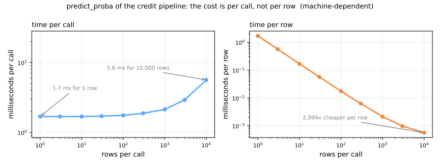
On the machine that built the page: 1.724 ms/row one at a time, 0.0006 ms/row in one batch, about 2,700×. A call costs about 1.7 ms whether it carries one row or a thousand: fixed work, not arithmetic.
Reproducibility: every ingredient has a version
| ingredient | what to record | typical tool |
|---|---|---|
| code | the commit that trained it | git |
| data | a fingerprint and a way to get the rows back | DVC, lakeFS, snapshots |
| environment | library versions | lock files, a container |
| randomness | every seed | random_state |
| configuration | hyperparameters, features, thresholds | a config file in git |
| results | metrics, the artifact | tracker, model registry |
Seeds: same score, different decisions
Two random forests that differ only in their seed:
AUC
probabilities
decisions
Fingerprint the data
training data      68ad024c9661
one value changed  7eb64a1901f0
rows shuffled      a662547f0332
same data again    68ad024c9661
- One changed value out of 6,000 gives a completely different fingerprint; so does another row order.
- "Was it trained on this month's extract?" becomes a string comparison.
A hash only identifies the data; rebuilding needs the rows themselves (DVC, lakeFS, read-only snapshots).
An experiment log: one line per run, never edited
| data | C | CV AUC | CV std |
|---|---|---|---|
| 68ad024c9661 | 0.01 | 0.7495 | 0.0292 |
| 68ad024c9661 | 0.10 | 0.7599 | 0.0224 |
| 68ad024c9661 | 1.00 | 0.7522 | 0.0244 |
| 68ad024c9661 | 10.00 | 0.7442 | 0.0230 |
C = 0.1 over C = 1 (0.0077) is far below the fold standard deviations (about 0.02): treat them as tied. Keep the losing runs: they record how many things were tried.Monitoring: models decay silently
The service keeps answering 200 OK while its predictions get worse. Three layers: system, data quality, statistical drift.
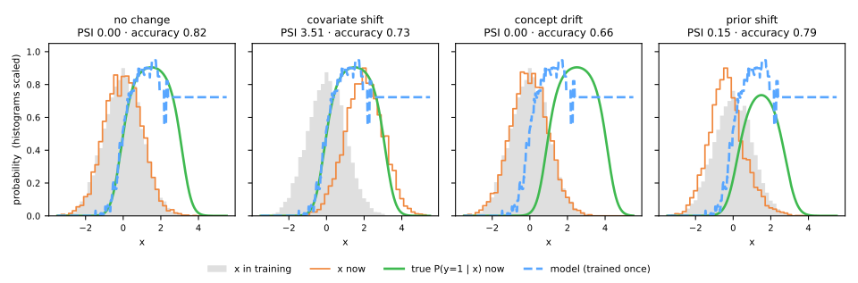
| shift | what changes | what stays fixed | example |
|---|---|---|---|
| covariate | \(P(x)\) | \(P(y \mid x)\) | the bank sells to younger clients |
| concept | \(P(y \mid x)\) | \(P(x)\) | a crisis changes who repays |
| prior | \(P(y)\) | \(P(x \mid y)\) | an epidemic: more patients are sick |
Measuring a shift: PSI, by hand
\[ \text{PSI} = \sum_{i=1}^{B} (a_i - e_i)\,\ln\frac{a_i}{e_i} \]| bin | \(e_i\) | \(a_i\) | \(\ln(a_i/e_i)\) | term |
|---|---|---|---|---|
| 1 | 0.25 | 0.10 | −0.916 | 0.1374 |
| 2 | 0.25 | 0.20 | −0.223 | 0.0112 |
| 3 | 0.25 | 0.30 | +0.182 | 0.0091 |
| 4 | 0.25 | 0.40 | +0.470 | 0.0705 |
| PSI | 0.228 |
Bins cut at the training quartiles. Every term is positive.
< 0.1 no meaningful change · 0.1–0.25 worth watching · > 0.25 significant (Siddiqi, 2006)
What does PSI = 0.25 mean?
| mean moved by | 0 | 0.1 sd | 0.25 sd | 0.5 sd | 1 sd |
|---|---|---|---|---|---|
| PSI (10 bins) | 0.005 | 0.015 | 0.064 | 0.250 | 0.929 |
The alarm level is a move of half a standard deviation. With no shift at all, PSI is not exactly zero: two samples never have identical histograms.
Simulator: PSI, bin by bin
Predict. Turn on concept drift without moving the inputs. What happens to PSI, and to the accuracy?
Measuring a shift: the KS test
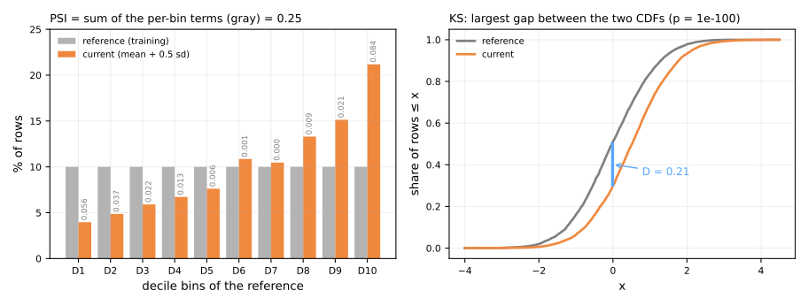
By hand, 1–5 against 3–7: \(D = 0.4\), \(p = 0.873\): not surprising with five points per side.
| a shift of 0.02 sd, n = | 1,000 | 10,000 | 100,000 | 1,000,000 |
|---|---|---|---|---|
| KS p-value | 0.097 | 0.14 | 0.00049 | 1.6e-41 |
| PSI | 0.0344 | 0.0018 | 0.0004 | 0.0005 |
The three shifts, measured
| PSI(x) | KS p | accuracy | precision | actual rate | mean predicted | |
|---|---|---|---|---|---|---|
| no change | 0.004 | 0.695 | 0.816 | 0.769 | 0.462 | 0.465 |
| covariate shift | 3.505 | 0.000 | 0.728 | 0.729 | 0.720 | 0.780 |
| concept drift | 0.003 | 0.340 | 0.660 | 0.329 | 0.167 | 0.459 |
| prior shift | 0.152 | 0.000 | 0.794 | 0.491 | 0.200 | 0.339 |
Labels arrive late: monitoring at two speeds
immediately
data-quality checks, PSI or KS of each input, and the distribution of the model's own scores: one of the most effective shift detectors, for one line (Rabanser et al., 2019)
later, with the outcomes
the real metrics (AUC, precision, calibration) per batch, against the validation estimate
Degrade, detect, retrain
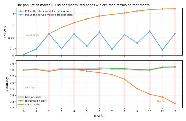
The population moves 0.3 sd per month. Static model vs a model retrained whenever its input PSI crosses 0.25.
| month | static | monitored | best possible |
|---|---|---|---|
| 0 | 0.801 | 0.801 | 0.802 |
| 2 (alert) | 0.780 | 0.780 | 0.785 |
| 6 | 0.759 | 0.814 | 0.830 |
| 8 | 0.654 | 0.822 | 0.816 |
| 12 | 0.273 | 0.849 | 0.850 |
Training–serving skew, measured
A new client application sends a field in different units. The test set, three ways:
| AUC | flagged | decisions changed | rejected by the schema | |
|---|---|---|---|---|
| as in training | 0.783 | 20.0% | 0.0% | 1% |
| amount in thousands | 0.775 | 14.8% | 5.2% | 100% |
| duration in years | 0.751 | 2.8% | 17.2% | 93% |
Shipping a new model safely
First an evaluation gate: beat the current model on recent labeled data neither saw, by more than the noise. Then roll out in stages:
| strategy | how | protects against |
|---|---|---|
| shadow | scores live traffic, answers only logged | crashes, latency, strange scores |
| canary | 1–5% of traffic | problems that only show with real users |
| A/B test | random split, a business metric | "better AUC" that is not better outcomes |
| rollback | the previous artifact stays ready | everything else, in minutes |
Tests, documentation, and maturity
The ML Test Score
28 tests in 4 groups: data, model development, infrastructure, monitoring (Breck et al., 2017). The score is the minimum over the groups.
Model card
intended use, factors, metrics, training and evaluation data, ethical considerations, caveats (Mitchell et al., 2019)
A sensible ladder
- script + versioned artifacts
- CI/CD: tests before any model ships
- logging, dashboards, drift alerts
- retraining with gates and rollback
Climb when the pain justifies it.
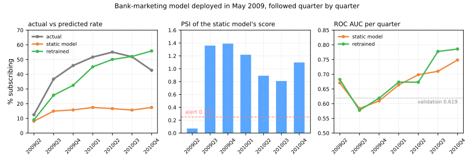
Shipping and monitoring a bank-marketing model
45,211 telemarketing calls, May 2008 to November 2010, in the order they were made. Deployed on 1 May 2009, followed for 19 months.
Build and validate (1–3), package and guard (4–6), monitor (7–9), retrain (10), write the model card (11).
The score PSI jumps above 0.8 from the second quarter: the cheapest and most useful single monitor.
Lab notebook (Jupyter or Colab, File → Upload notebook).
Summary
- Ship the whole pipeline, check the round trip, pin the versions; a pickle is a program.
- Put a schema in front of the model and answer with its version.
- Version code, data (a hash), environment, seeds and results.
- Monitor inputs and scores at once, outcomes later; PSI for magnitudes.
- Drift is not damage; concept drift needs labels.
- New models pass a gate and roll out in stages, with rollback ready.