Model Selection
You have met overfitting three times already: the degree-15 polynomial of the gradient descent lesson, the islands that k-nearest neighbors (k-NN) draws around single points when \(k = 1\) (the k-NN lesson), and the C curve of the cross-validation lab. The cross-validation lesson then gave you the machinery to choose honestly: cross-validation (CV), GridSearchCV, fold-by-fold comparisons, the one-standard-error rule and nested CV. This lesson does not repeat that machinery. It is about the why and the which way: why every model fails in one of two opposite directions, how to tell from the data which of the two you are in, and what to do about each.
The theory is the bias–variance decomposition, which we will not only state but measure, number by number, on a problem whose truth we know. The practical tools are validation curves and learning curves. The oldest trap is regression to the mean. And the lesson ends with a sobering result, no free lunch: no model family wins everywhere, so choosing among families is part of the job. Every number quoted below comes from the code blocks or from the figure scripts next to this page.
How this lesson is organized
The lesson has two approaches. Each has slides, text and a lab to do in class on Colab; the quiz at the end covers the fundamental one. Start with the fundamental approach: the advanced one builds on it.
| Fundamental approach | Advanced approach | |
|---|---|---|
| question | Is my model wrong because it is too rigid, or because it listens too closely to the sample? And what do I do in each case? | How to choose among model families without being fooled by luck |
| content | bias, variance and noise; the decomposition, measured; validation curves; learning curves; the diagnosis; the complexity knobs | effective number of parameters, regression to the mean, the family as a hyperparameter, no free lunch, Occam's razor, the whole workflow |
| in-class lab | house prices: diagnose and treat, steps 1 to 6 | select and test, steps 7 to 9 |
| by the end, you can | tell from two curves whether a model suffers from bias or from variance; predict whether more data will help; turn the right knob the right way | compare families in a single search; recognize a tie; distrust the winner's score; measure how precise the test score is |
Both labs use the same notebook on Colab (in Portuguese): the fundamental part runs from step 1 to 6, the advanced part from step 7 to 9. Everything runs in the browser; there is nothing to download.
Fundamental approach
One question drives this part: when a model is wrong, why is it wrong? There are only two possible directions, opposite to each other, and each has a remedy that makes the other one worse. This part measures both on a problem whose truth we know, then teaches how to recognize them, without knowing the truth, from two curves.
This part follows one pipeline in four stages, drawn below: 1. two ways to be wrong, underfitting and overfitting on many fits of one truth; 2. split the error into bias², variance and noise, measured; 3. diagnose with curves, validation and learning curves when the truth is unknown; 4. turn the knob, each family's complexity knob, put to work in the lab. Each stage links to its section, and in the slides a strip at the bottom shows which stage you are in.
- Two ways to be wrongmany fits of one truth: underfitting and overfitting
- Split the errorbias² + variance + noise, measured
- Diagnose with curvesvalidation curve, learning curve, the diagnosis
- Turn the knobeach family's complexity knob, then the lab: diagnose and treat
Fundamental approach slides
Click the slides and use the ← → arrows to navigate; F opens full screen and Esc shows every slide. Open the slides in a new tab
1. Two ways to be wrong
Stage 1. To see what a model gets wrong systematically, you would need something no real project has: many independent training sets drawn from the same source. On a problem we invent, we can have them. The truth is \(f(x) = \sin(2\pi x)\) on \([0, 1]\); a training set is 30 points \(x\) drawn at random, each with \(y = f(x)\) plus Gaussian noise of standard deviation 0.3. We draw five such training sets, fit polynomials of degree 1, 3 and 12 to each, and look at what every fitted model predicts at one point, \(x = 0.25\), where the truth is \(f(0.25) = 1\):
import numpy as np
from sklearn.linear_model import LinearRegression
from sklearn.pipeline import make_pipeline
from sklearn.preprocessing import PolynomialFeatures, StandardScaler


def f(x):                                          # the truth, which in real life nobody knows
    return np.sin(2 * np.pi * x)


def poly(degree):
    return make_pipeline(PolynomialFeatures(degree), StandardScaler(), LinearRegression())


rng = np.random.default_rng(0)
x0 = np.array([[0.25]])                            # the point we watch; f(0.25) = 1
print('training set   degree 1   degree 3   degree 12')
for s in range(5):
    x = rng.uniform(0, 1, 30)                      # a fresh sample of 30 points...
    y = f(x) + rng.normal(0, 0.3, 30)              # ...with noise of standard deviation 0.3
    preds = [poly(d).fit(x.reshape(-1, 1), y).predict(x0)[0] for d in (1, 3, 12)]
    print(f"{s + 1:12d}   " + '   '.join(f"{p:8.2f}" for p in preds))
training set   degree 1   degree 3   degree 12
           1       0.24       1.09       1.05
           2       0.57       1.05       1.06
           3       0.60       0.97       0.95
           4       0.39       1.18       1.29
           5       0.43       1.01       1.08
A worked example, by hand. Take the degree-1 column. The five predictions average to \((0.24 + 0.57 + 0.60 + 0.39 + 0.43)/5 = 0.446\). The truth is 1, so the straight line misses by \(0.446 - 1 = -0.554\) on average: that systematic miss is the bias, and its square is \(0.307\). Around their own average the five predictions scatter by \(-0.206, +0.124, +0.154, -0.056, -0.016\); the mean of the squares, \((0.0424 + 0.0154 + 0.0237 + 0.0031 + 0.0003)/5 = 0.017\), is the variance. For degree 3 the same arithmetic gives an average of 1.060, so a bias of only 0.060 (squared: 0.0036), and a variance of \((0.03^2 + 0.01^2 + 0.09^2 + 0.12^2 + 0.05^2)/5 = 0.0052\).
The two numbers answer two different questions. Bias: if I could average over every training set I might have been given, would I be right? Variance: how much does my answer depend on which training set I happened to get? The straight line is wrong at \(x = 0.25\) in the same way every time: it cannot bend. Degree 12 looks almost as good as degree 3 at this point, and that is a warning about looking at one point only. The figure below draws whole curves instead, 20 of them per degree, from the 500 training sets used in the next section (figure script):
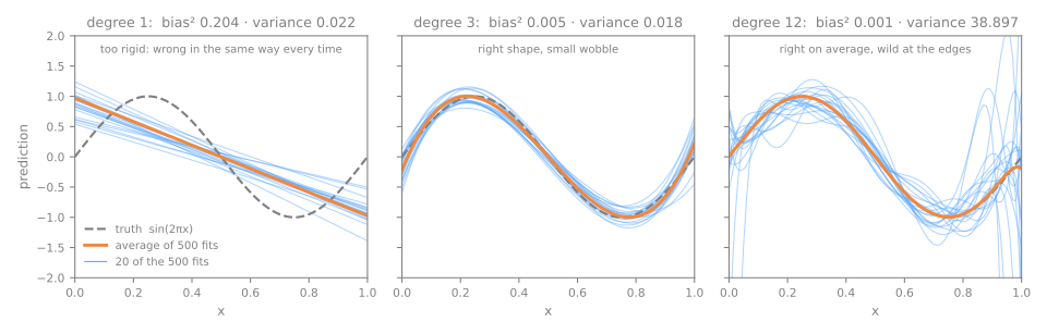
The degree-1 fits (left) agree with each other and are all wrong: high bias, low variance. The degree-12 fits (right) are right on average (the orange mean of 500 fits sits almost on the truth), yet any single one of them can be far off, especially near the edges, where a training set may happen to have no points and the polynomial is free to shoot up or down: low bias, high variance. Degree 3 (middle) has both small. The first failure is called underfitting, the second overfitting.
The classic picture of these two failures is a dartboard. Each dart is one model, trained on a different sample; the bullseye is the truth. Bias is the distance from the bullseye to the average of the darts; variance is how widely the darts scatter around that average. The labels use the numbers measured in the next section (figure script):
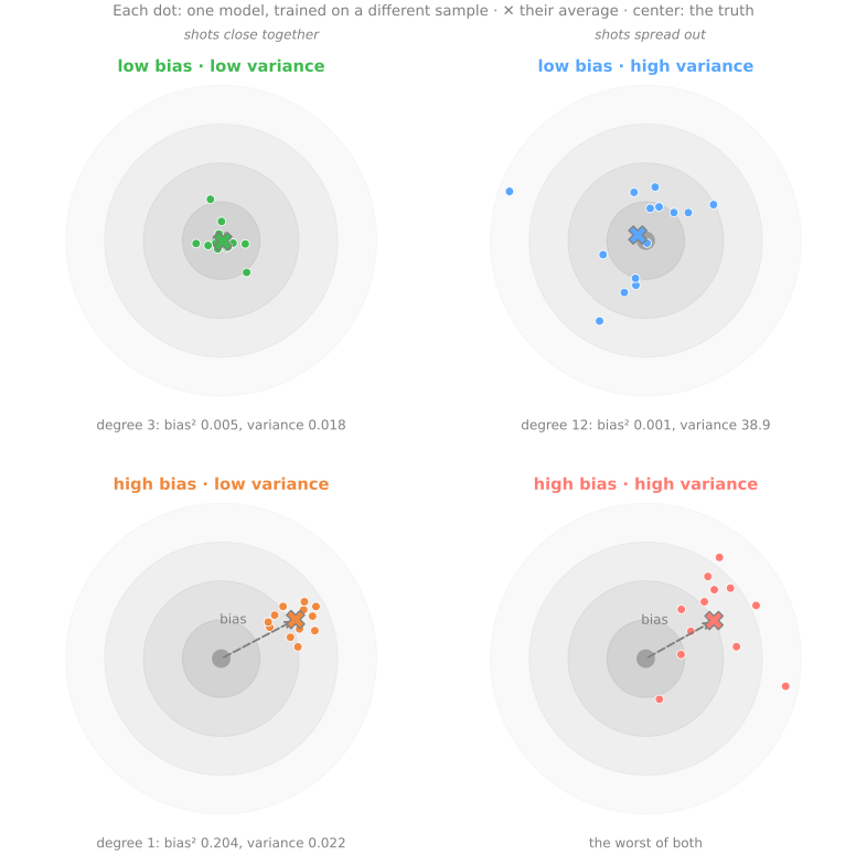
Look at the top-right board: the average of the darts hits the bullseye, yet no single dart can be trusted. That is the model that looks great "on average" and disappoints on the one training set you actually have.
2. The bias–variance trade-off
Stage 2. For squared error, the two quantities of the worked example, plus the noise, add up exactly to the expected test error. Fix a point \(x\). A new observation there is \(y = f(x) + \varepsilon\), with noise \(\varepsilon\) of mean 0 and variance \(\sigma^2\). The prediction \(\hat f(x)\) is random too, because it depends on the training set. Averaging over both:
Why it adds up, in two lines. First, \(y - \hat f = (f - \hat f) + \varepsilon\), and the new noise \(\varepsilon\) is independent of the training set and has mean 0, so the cross term vanishes and \(\mathbb{E}[(y - \hat f)^2] = \mathbb{E}[(f - \hat f)^2] + \sigma^2\). Second, for any random quantity \(Z\), \(\mathbb{E}[Z^2] = (\mathbb{E}[Z])^2 + \operatorname{Var}(Z)\) (the mean of the squares is the square of the mean plus the spread); with \(Z = f - \hat f\) that is bias² + variance. At \(x = 0.25\), the five training sets of the worked example put the expected error of degree 1 at about \(0.307 + 0.017 + 0.09 = 0.414\), and that of degree 3 at about \(0.0036 + 0.0052 + 0.09 = 0.099\).
- Bias is the error of the model family's best effort on average: a line cannot follow a sine, however many samples it sees;
- Variance is the price of listening to the particular sample: the more freedom the model has, the more its answer changes when the sample changes;
- Noise \(\sigma^2\) is the part of \(y\) that does not depend on \(x\) at all. Here \(\sigma^2 = 0.3^2 = 0.09\), and no model can go below it.
Measured, with 500 training sets
Five training sets give a rough idea; 500 give much steadier numbers. The function below trains a model on 500 fresh training sets, records its predictions on 101 points spread over \([0, 1]\), and also scores every fitted model on fresh test data, so that the decomposition can be checked against a direct measurement:
def bias_variance(make_model, n_sets=500, n=30, sigma=0.3, seed=0):
    """Train make_model() on n_sets fresh samples; split its test error into three parts."""
    rng = np.random.default_rng(seed)              # same seed -> every model sees the same samples
    x_grid = np.linspace(0, 1, 101)                # where we look at the predictions
    preds, test_mse = [], []
    for _ in range(n_sets):
        x = rng.uniform(0, 1, n)
        y = f(x) + rng.normal(0, sigma, n)
        p = make_model().fit(x.reshape(-1, 1), y).predict(x_grid.reshape(-1, 1))
        y_new = f(x_grid) + rng.normal(0, sigma, x_grid.size)     # fresh test data
        preds.append(p)
        test_mse.append(np.mean((y_new - p) ** 2))
    preds = np.array(preds)                                   # n_sets x 101
    bias2 = np.mean((preds.mean(axis=0) - f(x_grid)) ** 2)    # average curve vs truth
    variance = np.mean(preds.var(axis=0))                     # spread around the average curve
    return bias2, variance, sigma ** 2, np.mean(test_mse)


print('degree   bias²   variance   noise     sum   measured test MSE')
for d in [0, 1, 3, 5, 7, 9, 12]:
    b2, var, noise, mse = bias_variance(lambda: poly(d))
    print(f"{d:6d} {b2:7.3f} {var:10.3f} {noise:7.2f} {b2 + var + noise:7.3f} {mse:10.3f}")
degree   bias²   variance   noise     sum   measured test MSE
     0   0.495      0.020    0.09   0.605      0.603
     1   0.204      0.022    0.09   0.316      0.314
     3   0.005      0.018    0.09   0.113      0.112
     5   0.000      0.045    0.09   0.135      0.135
     7   0.001      0.635    0.09   0.726      0.723
     9   0.005      3.434    0.09   3.529      3.525
    12   0.001     38.897    0.09  38.987     38.985
How to read it:
- The columns add up. For every degree, bias² + variance + noise matches the test mean squared error (MSE) measured directly on fresh data, to within 0.004. That agreement cannot fail: the decomposition is an identity, so the two columns agree by construction, up to the noise of the fresh test draws. It is not a metaphor: it is arithmetic, and here you can watch it hold.
- Bias falls, then stays at zero. Degree 0 (a constant) has bias² 0.495; degree 1 cuts it to 0.204; from degree 3 on it is practically 0, because a cubic can already follow one period of a sine.
- Variance rises, slowly and then violently. 0.018 at degree 3, 0.045 at degree 5, 0.635 at degree 7, 38.897 at degree 12. With 30 points and 13 coefficients, one unlucky sample (a gap near an edge) is enough for the curve to shoot off. Read the large variances as orders of magnitude, not as precise values: a handful of the 500 samples produce most of them, so another seed changes those digits a lot. The U shape, and its bottom at degree 3, do not move.
- The sum is U-shaped, with its bottom at degree 3: 0.113, only 0.023 above the noise floor of 0.09. That is the best a polynomial can do with 30 points of this problem, and it is the answer model selection should find.
Here is the same experiment for all degrees from 0 to 12, and for the complexity knobs of two other families (figure script):
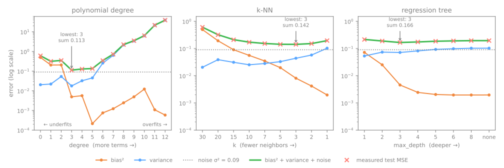
The same three families of curves, run with the same function:
from sklearn.neighbors import KNeighborsRegressor
from sklearn.tree import DecisionTreeRegressor

print('k-NN:  k   bias²   variance  test MSE')
for k in [30, 15, 7, 3, 1]:
    b2, var, noise, mse = bias_variance(lambda: KNeighborsRegressor(n_neighbors=k))
    print(f"{k:10d} {b2:7.3f} {var:10.3f} {mse:9.3f}")
print('tree: depth  bias²   variance  test MSE')
for depth in [1, 2, 3, 5, None]:
    b2, var, noise, mse = bias_variance(lambda: DecisionTreeRegressor(max_depth=depth, random_state=0))
    print(f"{str(depth):>11s} {b2:7.3f} {var:10.3f} {mse:9.3f}")
k-NN:  k   bias²   variance  test MSE
        30   0.495      0.020     0.603
        15   0.090      0.031     0.210
         7   0.035      0.028     0.152
         3   0.008      0.044     0.141
         1   0.002      0.102     0.195
tree: depth  bias²   variance  test MSE
          1   0.072      0.053     0.214
          2   0.025      0.073     0.188
          3   0.005      0.071     0.166
          5   0.002      0.093     0.185
       None   0.002      0.102     0.195
Three facts in this table can be predicted by hand, which is a good test of whether the decomposition makes sense to you:
- k-NN with \(k = 30\) is the degree-0 polynomial. With 30 training points, the 30 nearest neighbors of any \(x\) are all of them, so the prediction is the mean of \(y\), everywhere. Its numbers (bias² 0.495, variance 0.020, MSE 0.603) are those of degree 0 in the previous table. For k-NN the knob runs backwards: small \(k\) is the complex model, as you saw in the k-NN lesson.
- 1-NN has variance \(\approx \sigma^2\) and test error \(\approx 2\sigma^2\). Its prediction at \(x\) is the \(y\) of the nearest training point, that is, the truth near \(x\) plus that point's noise. So its variance is about the noise variance, 0.09 (measured: 0.102, a little more because the nearest point moves around), its bias is about zero (0.002), and its test error is about \(0.09 + 0.09 = 0.18\) (measured: 0.195): one dose of noise in the training label it copies, one in the test label.
- A fully grown tree is 1-NN, here. Without a depth limit, a regression tree on one feature keeps splitting until every leaf holds one training point, cutting halfway between neighboring \(x\) values: it predicts the \(y\) of the nearest point. Its row (0.002, 0.102, 0.195) is identical to 1-NN's. Trees get a lesson of their own (Decision Trees);
max_depthis their knob, and here depth 3 is best (0.166).
Every knob traces the same U. The families differ in how low the bottom of the U goes. In measured test MSE: 0.112 for the polynomial (degree 3), 0.141 for k-NN (\(k = 3\)), 0.166 for the tree (depth 3). A sine is smooth, and a smooth family wins on a smooth truth; on a different truth the order changes, which is the subject of section 10.
Drive the trade-off yourself. The simulator fits polynomials to 22 noisy points of the same sine and scores them on 22 others; slide from degree 0 (pure bias) to 12 (pure variance) and watch the two errors part ways:
3. Validation curves: the U from a single dataset
Stage 3. In a real project there is one dataset and no truth, so the decomposition cannot be computed. What you can compute is the sum, approximately: cross-validation estimates the test error of each setting. A validation curve does this for every value of one hyperparameter, and returns the training error too. This is the picture of the C curve in the cross-validation lesson, and scikit-learn has a function for it. On one sample of 30 points from the same sine, with 5-fold CV repeated 20 times to steady the estimate:
from sklearn.model_selection import RepeatedKFold, validation_curve

rng = np.random.default_rng(1)
x = rng.uniform(0, 1, 30)
y = f(x) + rng.normal(0, 0.3, 30)                  # ONE sample: all you ever get in practice
X = x.reshape(-1, 1)

degrees = np.arange(1, 11)
rcv = RepeatedKFold(n_splits=5, n_repeats=20, random_state=0)
train, val = validation_curve(poly(1), X, y, param_name='polynomialfeatures__degree',
                              param_range=degrees, cv=rcv, scoring='neg_mean_squared_error')
train, val = -train.mean(axis=1), -val.mean(axis=1)    # scikit-learn maximizes: MSE comes negated
print('degree  train MSE  validation MSE     gap')
for d, tr, va in zip(degrees, train, val):
    print(f"{d:6d} {tr:10.3f} {va:15.3f} {va - tr:7.3f}")
degree  train MSE  validation MSE     gap
     1      0.267           0.319   0.052
     2      0.246           0.386   0.140
     3      0.079           0.114   0.034
     4      0.070           0.311   0.241
     5      0.052           0.198   0.146
     6      0.049           0.255   0.206
     7      0.048           0.579   0.532
     8      0.047           0.424   0.377
     9      0.046           1.748   1.702
    10      0.046           1.222   1.176
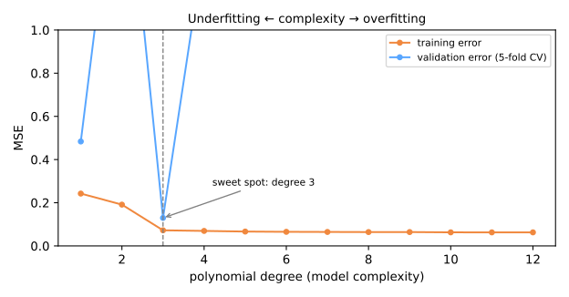
How to read a validation curve:
- The training curve only goes down (0.267 at degree 1, 0.046 at degree 10). More freedom always fits the sample you have better. It cannot see overfitting, and choosing by it would pick the most complex model every time.
- Left of the bottom: the bias side. At degrees 1 and 2 both errors are high (training 0.25–0.27, validation 0.32–0.39), and the gap between them is modest next to what comes later. The model is wrong on data it has seen almost as much as on data it has not.
- Right of the bottom: the variance side. Training error keeps falling while validation error climbs, to 1.748 at degree 9: the gap is the signature of variance.
- The bottom, degree 3 with 0.114, lands where the 500-sample decomposition put it. One sample of 30 points, a few lines of code, and the same answer as the simulation that knew the truth.
The figure adds a warning. The thin lines are the validation curves of 20 other samples of 30 points. On the left side they agree; on the right they scatter over three orders of magnitude (most of that range lies above the top of the plot, which is cut at 3), and even this sample's curve zigzags (0.311 at degree 4, 0.198 at degree 5). High-variance models do not just predict erratically, their validation scores are erratic too, because a single exploding fold dominates the mean. This is one more reason to prefer the simple end of a flat bottom, the one-standard-error rule of the cross-validation lesson.
4. Learning curves: is more data worth it?
A validation curve varies the complexity at a fixed amount of data. A learning curve does the opposite: it fixes the model and varies the number of training rows. It answers the most expensive question in a project: would more data help? Take one larger sample, 1,000 points of the same sine, and compare a model we know to be too rigid (degree 1) with one that has more freedom than 30 points can support (degree 9):
from sklearn.model_selection import KFold, learning_curve

rng = np.random.default_rng(3)
x = rng.uniform(0, 1, 1000)
y = f(x) + rng.normal(0, 0.3, 1000)
X = x.reshape(-1, 1)
cv = KFold(n_splits=5, shuffle=True, random_state=0)

for d in [1, 9]:
    sizes, train, val = learning_curve(poly(d), X, y, train_sizes=[15, 30, 60, 120, 250, 500, 800],
                                       cv=cv, scoring='neg_mean_squared_error')
    print(f"degree {d}   n: " + ' '.join(f"{n:7d}" for n in sizes))
    print("   train MSE: " + ' '.join(f"{v:7.3f}" for v in -train.mean(axis=1)))
    print("   valid MSE: " + ' '.join(f"{v:7.3f}" for v in -val.mean(axis=1)))
degree 1   n:      15      30      60     120     250     500     800
   train MSE:   0.182   0.254   0.243   0.273   0.248   0.255   0.269
   valid MSE:   0.301   0.275   0.279   0.279   0.271   0.270   0.270
degree 9   n:      15      30      60     120     250     500     800
   train MSE:   0.022   0.067   0.064   0.079   0.080   0.078   0.087
   valid MSE: 297.835   0.163   0.116   0.097   0.092   0.088   0.089
learning_curve trains on the first \(n\) rows of each training fold, for each \(n\) in train_sizes, and scores on the full validation fold. The figure shows the typical curves, computed from the known truth: for each size, the median over 300 training sets, with the middle half of them shaded (figure script):
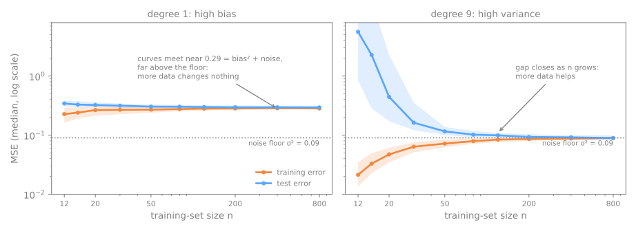
Two shapes, two diagnoses:
- High bias (degree 1). Training error rises with \(n\) (0.182 → 0.269: fitting 15 points is easier than fitting 800), validation error falls a little (0.301 → 0.270), and from about 120 points on the two stay within 0.03 of each other, ending at 0.269 and 0.270. More data changes nothing. The curves meet at the best a straight line can do, bias² + noise: about 0.29 in the figure, so about 0.2 above the noise floor of 0.09 (0.18 on this one sample). More data will not help; a more flexible model or better features will.
- High variance (degree 9). With 15 points and 10 coefficients the validation error is 297.835: the polynomial goes wild between points. It falls fast (0.163 at 30 points, 0.097 at 120) and reaches the noise floor (0.088–0.089) by 500 points, while the training error rises to meet it. The gap between the curves is the symptom of variance and, for a model with a fixed number of coefficients, data is what closes it. At 30 points this model is overfitting; at 800 it is the right model. This is the "too complex is relative to how much data you have" of the gradient descent lesson, now as a curve.
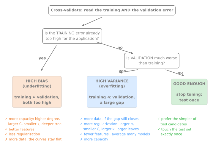
In practice the noise floor is unknown, so "high" has to mean something else: the error your application can tolerate, the error of a DummyRegressor baseline, or the error of the best model you have. What you look at is the shape: where the curves are heading, and whether the gap is still closing at the right edge of the plot. The lab does this on real data. The whole diagnosis fits in one table:
| what the curves show | diagnosis | helps | does not help |
|---|---|---|---|
| training ≈ validation, both too high, flat for large \(n\) | high bias (underfitting) | more capacity (higher degree, larger C, smaller k, deeper tree), better features, less regularization | more data; more regularization |
| training ≪ validation, gap still closing at the largest \(n\) | high variance (overfitting) | more data, more regularization (larger α, smaller C, larger k, min_samples_leaf), fewer features, averaging many models (Random Forest) | more capacity |
| training ≈ validation, both good enough | done | stop tuning | — |
The same diagnosis as a flowchart: two questions about the training and validation errors settle the case, and each outcome says what helps and what does not (figure script):
5. Every family has a complexity knob
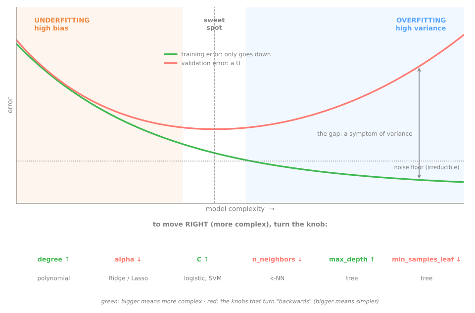
Stage 4. Every model family you have met has at least one hyperparameter that slides it along the U, from high bias to high variance. Some knobs are discrete (a degree), most are continuous (a penalty), and they do not all point the same way:
| model | knob | simpler (more bias, less variance) when | measured in |
|---|---|---|---|
| polynomial features | degree | smaller | the gradient descent lesson, this lesson |
| Ridge, Lasso | alpha | larger | the gradient descent lesson |
| logistic regression | C (inverse penalty) | smaller | the cross-validation lesson |
| k-NN | n_neighbors | larger | the k-NN lesson, this lesson |
| support vector machine (SVM), radial basis function (RBF) kernel | C, gamma | smaller C, smaller gamma | the SVM lesson |
| decision tree | max_depth, min_samples_leaf | smaller depth, larger leaves | this lesson, the decision trees lesson |
| gradient boosting | n_estimators, learning_rate, max_depth | fewer, smaller, shallower | the gradient boosting lesson |
| neural network | weight decay, training epochs | more decay, fewer epochs (early stopping) | the neural networks lesson |
"Regularization" in the narrow sense is the penalty on coefficient size of the gradient descent lesson. In the wide sense used by model selection, it is anything that restricts how freely a model can follow its training sample, and all of the knobs above qualify. Three of them run backwards and cause the most confusion: a larger alpha, a larger k and a larger min_samples_leaf make the model simpler, while a larger C, like a higher degree, makes it more complex.
One figure sums up the whole lesson: every model moves along the same complexity axis, and each family has its own knob to move along it (figure script):
6. Summary: the diagnosis in five lines
- Test error = bias² + variance + noise. The noise is a floor; the other two compete for the rest.
- Bias is being wrong the same way on every sample: training ≈ validation, both high. Variance is changing the answer with every sample: training ≪ validation.
- A validation curve varies complexity with the data fixed; a learning curve varies the data with the model fixed.
- For a model of fixed capacity, more data cures variance and not bias; more capacity only cures bias. Local models with a fixed \(k\) or leaf size are the exception: more data lowers their bias, and their variance stays. A wrong diagnosis spends resources on the wrong remedy.
- Every model has a complexity knob, and some turn backwards (
alpha,k,min_samples_leaf: bigger is simpler).
| symptom in the curves | diagnosis | what to do |
|---|---|---|
| training ≈ validation, both high, flat with more data | high bias | more capacity or better features |
| training ≪ validation, gap still closing | high variance | more data or more regularization |
| training error 0 (or 100% accuracy) on an unlimited model | memorization | limit the model; look only at validation |
| validation erratic across folds | high-variance model, unstable score | prefer the simple end of a flat bottom |
Fundamental lab — diagnose and treat
The problem. Each of the 20,640 rows is a district of California in the 1990 census, described by its location, the age of its houses, counts of rooms, bedrooms, people and households, the median income of its residents and its distance to the ocean. The target is the district's median house value. It is the instructor's copy of the dataset used throughout the course (Pace & Barry, 1997, in the version with missing values and an ocean_proximity column). The questions of this lab are the questions of this lesson: for three model families, is the error bias or variance? Would more data help? What fixes each diagnosis? And which model do we ship?
The workflow is the one from the validation lesson: lock away a test set, use one cv object for everything, and touch the test set exactly once, at step 9. This part does the diagnosis (steps 3 and 4) and treats each failure (steps 5 and 6); selection and testing are left to the advanced lab.
How to do this lab in class (about 40 min, in pairs)
- Open the lab notebook on Colab (in Portuguese). There is nothing to download or install: Colab runs in the browser. To keep your answers, save a copy to your Drive (File → Save a copy in Drive) before editing. Run the cells in order, in a single session.
- This lab is steps 1 to 6 of the notebook. The advanced lab continues in the same notebook, from step 7.
- Every step starts with a Predict: answer it with your partner before running the cell. Getting the prediction wrong is what makes the result memorable.
- After running, compare with the output and the reading on this page. Every output here is exactly what the code prints.
- The Simulations ask you to write a small Python experiment: change one input and watch what happens to the output. No hand calculations. The solution is collapsed right below: try before opening it.
- Suggested pace: steps 1 to 3 and the first simulation in 15 min; steps 4 to 6 and the second simulation in 25 min. Steps 4 and 5 take a few seconds each to run.
Step 1 — load and look
Predict. The target is the median house value of each district. Do you expect a symmetric distribution or a long tail? And if the census had a cap on high values, what would that do to the error of any model?
import numpy as np
import pandas as pd

url = 'https://raw.githubusercontent.com/hsandmann/biblio/refs/heads/main/ml/aula02/housing.csv'
df = pd.read_csv(url)
print(df.shape)
print(df.isna().sum()[lambda s: s > 0])
print(df['median_house_value'].describe().round(0))
print('districts at the 500,001 cap:', (df['median_house_value'] >= 500_001).sum())
(20640, 10)
total_bedrooms    207
dtype: int64
count     20640.0
mean     206856.0
std      115396.0
min       14999.0
25%      119600.0
50%      179700.0
75%      264725.0
max      500001.0
Name: median_house_value, dtype: float64
districts at the 500,001 cap: 965
20,640 districts and 10 columns. Only total_bedrooms has missing values (207 rows); an imputer in the pipeline will take care of them. The target has a mean of $206,856 and a median of $179,700, with a long right tail, and a detail worth knowing before any model is trained: 965 districts sit exactly at $500,001. The census recorded "more than $500,000" as that one value, so for those districts the true value is unknown and every model is scored against a number that is not the real price. They inflate the errors below, but not equally: a linear model, which cannot level off at a cap, pays for them more than a tree, which can.
Step 2 — lock the test set away, one cv for everything
Predict. The baseline predicts the same price for every district. Its root mean squared error (RMSE) should be close to which statistic of the prices you saw in step 1?
from sklearn.compose import ColumnTransformer
from sklearn.dummy import DummyRegressor
from sklearn.impute import SimpleImputer
from sklearn.model_selection import KFold, cross_validate, train_test_split
from sklearn.pipeline import make_pipeline
from sklearn.preprocessing import FunctionTransformer, OneHotEncoder, StandardScaler

X = df.drop(columns='median_house_value')
y = df['median_house_value']
X_train, X_test, y_train, y_test = train_test_split(X, y, test_size=0.2, random_state=42)

counts = ['total_rooms', 'total_bedrooms', 'population', 'households']      # skewed: log them
others = ['longitude', 'latitude', 'housing_median_age', 'median_income']
pre = ColumnTransformer([
    ('counts', make_pipeline(SimpleImputer(strategy='median'), FunctionTransformer(np.log1p),
                             StandardScaler()), counts),
    ('others', StandardScaler(), others),
    ('ocean', OneHotEncoder(handle_unknown='ignore'), ['ocean_proximity']),
])
cv = KFold(n_splits=5, shuffle=True, random_state=42)                      # one cv for everything


def rmse(model):
    """Mean training and validation RMSE over the 5 folds, and the fold std of validation."""
    r = cross_validate(model, X_train, y_train, cv=cv, return_train_score=True,
                       scoring='neg_root_mean_squared_error')
    return abs(r['train_score'].mean()), abs(r['test_score'].mean()), r['test_score'].std()


print(X_train.shape, X_test.shape)
print('dummy (predicts the mean): train %.0f · validation %.0f ± %.0f' % rmse(DummyRegressor()))
16,512 districts for development, 4,128 locked away until step 9. Everything that learns from data lives in the pre transformer, so cross-validation refits it inside every fold: the median used to fill total_bedrooms, the scalers, and the list of ocean_proximity categories. The four count columns are summed over a whole district and range from a handful to tens of thousands, so they are log-transformed first (log1p): a few huge districts would otherwise dominate the scale and, later, the polynomial features. The cv object is created once and used by every step, so every number below is measured on the same five folds.
scikit-learn maximizes scores, so it reports RMSE with a minus sign (neg_root_mean_squared_error); abs() turns it back into dollars. The baseline predicts the mean price for every district and misses by $114,793 on average (in the RMSE sense): that is simply the standard deviation of prices. Any model must be read against it.
Step 3 — three families, one first diagnosis
Predict. An unlimited-depth tree and a linear regression: which will have the lowest training error? And the largest gap between training and validation?
from sklearn.linear_model import LinearRegression
from sklearn.neighbors import KNeighborsRegressor
from sklearn.tree import DecisionTreeRegressor

candidates = {
    'linear': make_pipeline(pre, LinearRegression()),
    'k-NN (k=5)': make_pipeline(pre, KNeighborsRegressor()),
    'tree (no limits)': make_pipeline(pre, DecisionTreeRegressor(random_state=42)),
}
print(f"{'':17s} {'train':>7s} {'valid':>7s} {'gap':>7s}")
for name, model in candidates.items():
    tr, va, sd = rmse(model)
    print(f"{name:17s} {tr:7.0f} {va:7.0f} {va - tr:7.0f}")
One table, three different pictures:
- Linear regression: training 66,369, validation 66,460, a gap of only $91. It performs as badly on the districts it was fitted on as on new ones. That is the signature of high bias: it has cut the baseline error by 42%, and it has nothing left to learn with a linear function of these features.
- Unlimited tree: training RMSE 0. The tree grew until every leaf reproduced its training districts exactly, then missed new ones by 67,266. A gap of $67,266 is high variance in its purest form.
- k-NN with the default \(k = 5\): the best validation score of the three (59,967), with a clear gap of $11,069: some variance.
A single number per model (the validation RMSE) would rank them k-NN, linear, tree and stop there. The gap says why each one fails, and so what to try next. It does not yet say whether more data would help: that is the job of the next step.
Simulation: variance, up close. The gap between training and validation is a symptom; variance is the cause: how much the model changes when the sample changes. Measure it directly. Split X_train into three disjoint parts, A, B and C; train each family twice, once on A and once on B, and compare the predictions of the two versions on the same districts of C. Which family changes most from one sample to another?
Solution
from sklearn.base import clone

parts = np.array_split(np.random.default_rng(0).permutation(len(X_train)), 3)
(XA, yA), (XB, yB), (XC, yC) = [(X_train.iloc[p], y_train.iloc[p]) for p in parts]
print(f"three disjoint parts of {len(XA)}, {len(XB)} and {len(XC)} districts")
for name, model in candidates.items():
    pa = clone(model).fit(XA, yA).predict(XC)          # version trained on part A
    pb = clone(model).fit(XB, yB).predict(XC)          # version trained on part B
    err = np.sqrt(np.mean((yC - pa) ** 2))
    shift = np.sqrt(np.mean((pa - pb) ** 2))
    print(f"{name:17s} RMSE on C {err:6.0f} · A and B versions differ by {shift:6.0f}")
three disjoint parts of 5504, 5504 and 5504 districts
linear            RMSE on C  65458 · A and B versions differ by   4405
k-NN (k=5)        RMSE on C  62645 · A and B versions differ by  38519
tree (no limits)  RMSE on C  72083 · A and B versions differ by  79944
The two versions of the linear regression differ by US$ 4,405 (as a root mean square, RMS) on the same districts: changing the sample barely moves the line. The two versions of the unlimited tree differ by US$ 79,944, more than the error of either one (US$ 72,083): each tree memorized its own part, noise included, and the noise of A is not the noise of B. k-NN sits in between (US$ 38,519). This is the definition of variance from section 1, now on a real dataset: you did not need to know the truth to see it, two samples were enough. Notice also that with a third of the data the tree and k-NN make larger errors than in step 3 (72,083 and 62,645, against 67,266 and 59,967), while the linear regression stays where it was: exactly what the learning curves of the next step will show.
Step 4 — learning curves: would more data help?
Predict. The linear model already makes almost the same error on training and on validation. Will doubling the number of districts lower its validation error? And that of the unlimited tree?
import matplotlib.pyplot as plt
from sklearn.model_selection import learning_curve

fractions = [0.02, 0.05, 0.1, 0.2, 0.4, 0.7, 1.0]
fig, axes = plt.subplots(1, 3, figsize=(12, 3.5), sharey=True)
for ax, (name, model) in zip(axes, candidates.items()):
    sizes, train, val = learning_curve(model, X_train, y_train, train_sizes=fractions, cv=cv,
                                       scoring='neg_root_mean_squared_error')
    train, val = np.abs(train.mean(axis=1)), np.abs(val.mean(axis=1))
    print(f"{name:17s} n     " + ' '.join(f"{n:6d}" for n in sizes))
    print(f"{'':17s} train " + ' '.join(f"{v / 1000:6.1f}" for v in train))
    print(f"{'':17s} valid " + ' '.join(f"{v / 1000:6.1f}" for v in val))
    ax.plot(sizes, train, 'o-', label='training')
    ax.plot(sizes, val, 'o-', label='validation')
    ax.set_title(name)
    ax.set_xlabel('training rows')
axes[0].set_ylabel('RMSE (US$)')
axes[0].legend()
plt.show()
linear            n        264    660   1320   2641   5283   9246  13209
                  train   59.2   64.4   66.2   66.4   65.9   66.5   66.4
                  valid   67.8   67.6   67.0   66.8   66.5   66.5   66.5
k-NN (k=5)        n        264    660   1320   2641   5283   9246  13209
                  train   59.0   56.5   54.8   52.5   50.8   50.1   48.9
                  valid   78.0   72.0   69.3   65.8   62.9   61.3   60.0
tree (no limits)  n        264    660   1320   2641   5283   9246  13209
                  train    0.0    0.0    0.0    0.0    0.0    0.0    0.0
                  valid   91.5   85.6   83.9   77.5   72.7   71.8   67.3
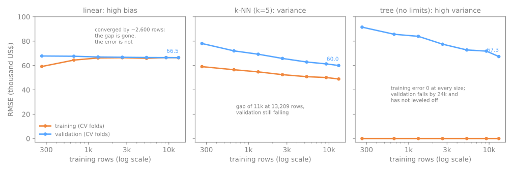
The table and the figure show the same numbers, in thousands of dollars:
- Linear: more data is useless. The training error rises from 59.2 to 66.4 and the validation error falls from 67.8 to 66.5; by 2,641 rows they have met (66.4 and 66.8), and the last 10,000 rows change nothing. The model has learned everything a hyperplane can learn from these features. Collecting more districts would cost money and buy nothing; the remedy is more flexibility (step 6).
- k-NN: more data would help. Validation falls from 78.0 to 60.0 and is still falling at the right edge (61.3 → 60.0 over the last 4,000 rows), while an 11,000-dollar gap remains. Denser data means closer neighbors, so less bias. With \(k\) fixed, each prediction still averages only 5 noisy prices, so that part of the variance stays: a larger \(k\) attacks it (step 5).
- Tree: more data would help, slowly. Training error is 0 at every size, and validation falls from 91.5 to 67.3, still dropping. Validation falls because, with more districts, finer leaves follow the truth more closely (less bias). But a leaf holding one district copies that district's noise at any size, so the gap can shrink but never close: its variance has a floor about the size of the noise. Regularization is the remedy (step 5).
Data is not the only thing in short supply. What the curves say is which resource to spend: engineering effort on features for the linear model, regularization for the other two (more data still lowers their error, but does not close their gap).
Step 5 — validation curves: treat the variance
Predict. Requiring more districts in every leaf of the tree: will it raise or lower the training error? And the validation error: does it always move the same way, or first one way and then the other?
from sklearn.model_selection import validation_curve

knobs = {'tree': (candidates['tree (no limits)'], 'decisiontreeregressor__min_samples_leaf',
                  [1, 2, 5, 10, 20, 50, 100]),
         'k-NN': (candidates['k-NN (k=5)'], 'kneighborsregressor__n_neighbors', [1, 3, 5, 10, 20, 50])}
for name, (model, param, values) in knobs.items():
    train, val = validation_curve(model, X_train, y_train, param_name=param, param_range=values,
                                  cv=cv, scoring='neg_root_mean_squared_error')
    print(f"{name}: {param.split('__')[1]}")
    for v, tr, va in zip(values, np.abs(train.mean(axis=1)), np.abs(val.mean(axis=1))):
        print(f"  {v:4d}   train {tr:6.0f}   valid {va:6.0f}   gap {va - tr:6.0f}")
tree: min_samples_leaf
     1   train      0   valid  67266   gap  67266
     2   train  18723   valid  64812   gap  46089
     5   train  34461   valid  60469   gap  26008
    10   train  43023   valid  57796   gap  14773
    20   train  49663   valid  58079   gap   8415
    50   train  56655   valid  59891   gap   3236
   100   train  61413   valid  63505   gap   2092
k-NN: n_neighbors
     1   train      0   valid  73873   gap  73873
     3   train  43627   valid  61904   gap  18277
     5   train  48898   valid  59967   gap  11069
    10   train  53606   valid  59182   gap   5576
    20   train  57036   valid  59931   gap   2895
    50   train  61204   valid  62371   gap   1168
Both tables have the U shape of this lesson, read along the gap column:
- Tree. Requiring at least
min_samples_leafdistricts in every leaf forces each prediction to be an average, and averages have less variance. The gap shrinks steadily (67,266 → 14,773 at 10 → 2,092 at 100) while validation error first falls and then rises again: the bottom ismin_samples_leaf = 10, 57,796. One knob took the tree from the worst of the three models to the best, a gain of $9,470. At 100 districts per leaf the tree has crossed to the bias side (small gap, 63,505). - k-NN. \(k = 1\) memorizes (training 0, validation 73,873); \(k = 50\) is on the bias side (gap 1,168, validation 62,371). The bottom is \(k = 10\) with 59,182, only $785 better than the default \(k = 5\): here the default was already near the bottom of a flat U.
Step 6 — treat the bias of the linear model
Predict. Adding the squares and products of the features to the linear model should lower the training error, the validation error, or both? What can go wrong with cubic terms?
from sklearn.linear_model import Ridge
from sklearn.preprocessing import PolynomialFeatures

print('degree   alpha    train    valid  ± std')
for degree, alpha in [(1, 1), (2, 1), (3, 0.1), (3, 10), (3, 100)]:
    model = make_pipeline(pre, PolynomialFeatures(degree), StandardScaler(), Ridge(alpha=alpha))
    tr, va, sd = rmse(model)
    print(f"{degree:6d} {alpha:7g} {tr:8.0f} {va:8.0f} {sd:6.0f}")
degree   alpha    train    valid  ± std
     1       1    66369    66460   1597
     2       1    58649    59741   1823
     3     0.1    52092    63828   7751
     3      10    53038    57510   2955
     3     100    54582    57473   2381
The linear model needs flexibility, and PolynomialFeatures provides it: degree 2 adds the squares and pairwise products of the 13 preprocessed columns, degree 3 the cubic terms too (560 columns in all). Read the rows in order:
- Degree 2 lowers both errors, training 66,369 → 58,649 and validation 66,460 → 59,741. The whole curve moved down: that is what reducing bias looks like.
- Degree 3 with a weak penalty (
alpha = 0.1) overshoots to the variance side: training 52,092, validation 63,828, and a fold standard deviation of 7,751, four to five times that of degrees 1 and 2, because on some folds the cubic terms extrapolate wildly for a few unusual districts. - Degree 3 with
alpha = 100keeps the capacity and lets the penalty take back what the data cannot support: validation 57,473 ± 2,381, the best number so far.
Degree adds capacity; alpha removes it continuously. Used together they are the two hands of the bias–variance trade-off, which is why "polynomial features + Ridge" is a standard recipe. Note what did not happen: no new data was needed.
Simulation: alpha as a continuous knob. Step 6 tried three values of alpha for degree 3. Sweep it from 0.01 to 1,000,000 (eight orders of magnitude) and follow training, validation, the gap between them and the fold standard deviation. At which end is the model on the variance side, and at which on the bias side?
Solution
print('alpha      train    valid    gap  ± std')
for alpha in [0.01, 1, 100, 1e4, 1e6]:
    tr, va, sd = rmse(make_pipeline(pre, PolynomialFeatures(3), StandardScaler(), Ridge(alpha=alpha)))
    print(f"{alpha:<8g} {tr:7.0f} {va:8.0f} {va - tr:6.0f} {sd:6.0f}")
alpha      train    valid    gap  ± std
0.01       51931    66098  14167   8694
1          52426    60366   7940   5378
100        54582    57473   2890   2381
10000      66352    66926    574   1330
1e+06     106790   106832     42   1318
Read the gap column from top to bottom: 14,167 → 42. With alpha = 0.01 the 560 terms are almost free: training 51,931, validation 66,098 and a fold standard deviation of 8,694, the variance side. With alpha = 1e6 the penalty crushes almost every coefficient: training and validation meet at about US$ 106,800, close to the baseline's 114,793, with a gap of US$ 42 — the bias side. The bottom of the U is at alpha = 100 (57,473). Same degree, same features: alpha alone carried the model from one end of the U to the other. And this knob turns "backwards": a larger alpha is a simpler model.
To close the fundamental part. In one sentence each: (1) what does the gap between training and validation error measure, and what does it not measure? (2) Why would more districts not help the linear model of step 4? (3) Which knob would you turn, and which way, to take the tree off the variance side?
Your turn (fundamental)
At home:
- More points. Rerun the
bias_varianceof section 2 for polynomials withn=100instead of 30. Which degree is best now, and what happened to the variance of degree 12? Relate the answer to the learning curves. - More noise. Rerun it with
sigma=0.6. Does the best degree move toward simpler or more complex models? Explain with the three terms of the decomposition. - Features against bias. Add three ratios to
Xbefore the split: rooms per household, bedrooms per room and people per household (they need a small change tocounts/others). Rerun step 6. Does the degree-1 model's plateau move, and by more than one fold standard deviation?
Advanced approach
The fundamental part taught how to diagnose and treat one model. This part is about choosing among many: what selection does to its own scores (regression to the mean), how to compare whole families in a single search, why no family wins everywhere, and how to break a tie when the data cannot. The code blocks continue those of sections 1 to 5.
This part follows one pipeline in four stages: 1. a common scale for complexity, the effective number of parameters; 2. regression to the mean, why the winner's score falls when measured again; 3. compare families in one search, with no free lunch and Occam's razor; 4. the whole workflow, with a one-way door before the test, and the lab. Each stage links to its section, and in the slides a strip at the bottom shows which stage you are in.
- A common scalethe effective number of parameters
- Regression to the meanwhy the winner's score falls when measured again
- Compare familiesone search over all families, no free lunch, Occam's razor
- The whole workflowfive steps, a one-way door before the test, then the lab
Advanced approach slides
Click the slides and use the ← → arrows to navigate; F opens full screen and Esc shows every slide. Open the slides in a new tab
7. A common scale: the effective number of parameters
Stage 1. The knobs can even be put on a common scale. For models whose predictions on the training points are a weighted sum of the training labels, the effective number of parameters is the sum, over the training points, of the weight each point's own label gets in its own prediction (Hastie, Tibshirani & Friedman, ch. 7). For least squares with \(p\) columns that sum is \(p\). For k-NN, every training point is one of its own \(k\) nearest neighbors and gets weight \(1/k\), so the total is \(n/k\): with 30 points, \(k = 30\) spends 1 parameter (the mean, the degree-0 polynomial: same numbers in the table above), \(k = 3\) spends 10, and \(k = 1\) spends 30, one per data point, which is memorization. For Ridge, the effective number of parameters falls continuously from \(p\) toward 1 as \(\alpha\) grows (the 1 is the intercept, which is not penalized). This is why a penalty is such a convenient knob: it turns the staircase of degrees into a slope.
8. Regression to the mean
Stage 2. Francis Galton gave regression its name in 1886, puzzled that very tall parents had children closer to average height; the story, the data and a simulator are in the linear regression lesson. The mechanism deserves a second look here, because model selection runs into it every time it picks a winner.
Any measured performance is part skill and part luck. Simulate 10,000 students whose true ability has mean 70 and standard deviation 8, and let each exam add a day's luck. Select the top 10% on a first exam, and look at the same students on a second one, for three levels of luck:
rng = np.random.default_rng(0)
n = 10_000
ability = rng.normal(70, 8, n)                     # what each student really knows (sd 8)
print('luck sd   r = 8²/(8²+luck²)   top 10% on exam 1   same students, exam 2   predicted')
for luck in [2, 6, 16]:
    exam1 = ability + rng.normal(0, luck, n)       # one day's luck...
    exam2 = ability + rng.normal(0, luck, n)       # ...and another day's
    top = exam1 >= np.quantile(exam1, 0.9)
    r = 8 ** 2 / (8 ** 2 + luck ** 2)
    predicted = exam1.mean() + r * (exam1[top].mean() - exam1.mean())
    print(f"{luck:7d} {r:19.2f} {exam1[top].mean():19.1f} {exam2[top].mean():23.1f} {predicted:11.1f}")
luck sd   r = 8²/(8²+luck²)   top 10% on exam 1   same students, exam 2   predicted
      2                0.94                84.4                    83.5        83.6
      6                0.64                87.6                    80.9        81.3
     16                0.20               101.4                    76.1        76.3
Nobody's ability changed between the exams, and yet the top group falls every time. How far it falls can be computed in advance. The share of the spread in scores that is ability rather than luck is the reliability, \(r = \sigma^2_\text{ability} / (\sigma^2_\text{ability} + \sigma^2_\text{luck})\). A group selected at a distance \(D\) above the mean on the first measurement is expected at \(r \times D\) above it on the second. With luck of standard deviation 6: \(r = 64/100 = 0.64\), the top group scored 87.6, that is 17.6 above the mean of 70, so the expectation is \(70 + 0.64 \times 17.6 \approx 81.3\); the simulation gives 80.9. With little luck (\(r = 0.94\)) the top group barely moves, 84.4 → 83.5. With a lot (\(r = 0.20\)) most of the lead was luck, 101.4 → 76.1 (figure script):
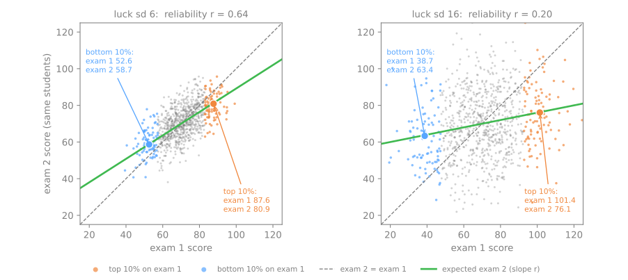
The effect runs in both directions: the bottom 10% improve, from 52.6 to 58.7 (and from 38.7 to 63.4 with heavy luck), with no help from anyone. An extreme score is extreme partly because the luck was extreme, and luck does not repeat. This is why the athlete on the magazine cover has a worse next season, why the fund with the best return of the year usually disappoints the next one, and why a remedial class for the worst scorers "works" even if it teaches nothing.
Now translate to model selection. A configuration is a student; its true performance on future data is its ability; its cross-validation score is one exam, whose luck comes from which rows fell in which fold and from which sample of the world you happened to collect; the winner of a grid search is the top of the class. Reliability is lowest exactly where selection happens: near the top of a grid, the configurations differ very little from each other (small spread of ability), while the CV noise does not shrink (same luck). So the winner's score regresses, and the more candidates you compare, the more extreme, and luckier, the winner. The cross-validation lesson measured the extreme case: on pure noise every configuration has the same ability, \(r = 0\), and the winner of 100 validation scores fell from 61.2% all the way back to 50.9% on the test set. Nested cross-validation measured a mild case on real data, a winner's 0.712 regressing to about 0.70.
Selection inflates scores; re-measurement deflates them
As a rule of thumb, the best of many noisy scores overestimates its own true score by roughly \((1 - r)\) times its lead over the pack (a heuristic: it assumes independent noise, and neighboring configurations of a grid share most of theirs). Never report the score that was used to pick the winner. Re-measure it on data that played no part in the choice: the locked test set or nested CV. Re-running CV with different folds on the same data is not enough: it shows how much of the ranking is fold luck (lab, step 8), but the winner was still chosen on these rows. And when something is done because a score was extreme (retrain only the worst segment, reward only the best team), expect some improvement or decline from regression to the mean alone: only a comparison group can separate it from the effect of what you did.
9. Grid search with cross-validation: the family as a hyperparameter
Stage 3. The mechanics are in the cross-validation lesson: wrap the preprocessing and the model in a pipeline, give GridSearchCV a grid and one cv object, read best_params_ and cv_results_, compare candidates fold by fold, prefer the simpler one when they tie, and grade the winner on data it has never seen. validation_curve, above, is a grid search over a single hyperparameter that also returns the training scores (in GridSearchCV you ask for them with return_train_score=True).
One extension is worth knowing: the model family can itself be a hyperparameter. A pipeline step is a slot, and a grid can put different estimators in it. Passing a list of grids lets each family bring its own knobs, and 'passthrough' removes a step where a family does not need it (a tree does not care about scaling). Here are four families in one search, on the radar returns of the SVM lab:
import pandas as pd
from sklearn.datasets import fetch_openml
from sklearn.linear_model import LogisticRegression
from sklearn.model_selection import GridSearchCV, StratifiedKFold
from sklearn.neighbors import KNeighborsClassifier
from sklearn.pipeline import Pipeline
from sklearn.svm import SVC
from sklearn.tree import DecisionTreeClassifier

pipe = Pipeline([('scale', StandardScaler()), ('model', LogisticRegression())])  # 'model' is a slot
param_grid = [                                     # a list of grids: one per family
    {'model': [LogisticRegression(max_iter=5000)], 'model__C': np.logspace(-3, 3, 7)},
    {'model': [KNeighborsClassifier()], 'model__n_neighbors': [1, 3, 5, 9, 15, 25, 51]},
    {'model': [SVC()], 'model__C': [0.1, 1, 10, 100], 'model__gamma': ['scale', 0.01, 0.1]},
    {'model': [DecisionTreeClassifier(random_state=0)], 'scale': ['passthrough'],
     'model__max_depth': [1, 2, 3, 4, 6, 8, 12, None]},
]
cv = StratifiedKFold(n_splits=5, shuffle=True, random_state=0)
search = GridSearchCV(pipe, param_grid, cv=cv, scoring='accuracy', n_jobs=-1)

FAMILY = {'LogisticRegression': 'logistic', 'KNeighborsClassifier': 'k-NN',
          'SVC': 'SVM', 'DecisionTreeClassifier': 'tree'}


def best_per_family(search):
    """The best configuration of each family, read from cv_results_."""
    res = pd.DataFrame(search.cv_results_)
    res['family'] = [FAMILY[type(p['model']).__name__] for p in res['params']]
    best = res.loc[res.groupby('family')['mean_test_score'].idxmax()]
    best['setting'] = [', '.join(f"{k.split('__')[1]}={v}" for k, v in p.items() if '__' in k)
                       for p in best['params']]
    return best.set_index('family')[['mean_test_score', 'std_test_score', 'setting']]


ion = fetch_openml(data_id=59, as_frame=True)                # 351 radar returns, 34 features
X_ion, y_ion = ion.data, (ion.target == 'g').astype(int)
search.fit(X_ion, y_ion)
print(len(search.cv_results_['params']), 'configurations, 4 families, one search')
print(best_per_family(search).round(3).to_string())
34 configurations, 4 families, one search
          mean_test_score  std_test_score           setting
family
SVM                 0.946           0.037  C=10, gamma=0.01
k-NN                0.866           0.034     n_neighbors=1
logistic            0.883           0.035            C=10.0
tree                0.897           0.040       max_depth=2
One search, 34 configurations, 170 fits, and each family's best configuration read back from cv_results_. The kernel SVM wins, 0.946 against 0.897 for the best tree, in line with the SVM lab, where switching to an RBF kernel was the largest gain on this data. Because every configuration was scored on the same cv, the per-fold scores of any two families (split0_test_score, …) can be compared fold by fold straight from cv_results_. What does not change: best_score_ is still the best of 34 noisy estimates, so it carries the winner's curse of the previous section, and in a real project the search runs on the training part only, with a test set locked away (as in the lab).
A grid's cost multiplies with every hyperparameter you add. RandomizedSearchCV has the same interface but tries a fixed number n_iter of combinations drawn at random from distributions you give it (for example loguniform(1e-3, 1e3) for C): its cost no longer depends on how finely you describe the space, and because usually only a few hyperparameters really matter, random combinations cover those few much better than a grid does (Bergstra & Bengio, 2012). Smarter searches, which learn from the configurations already tried (successive halving, Bayesian optimization with Optuna), are the subject of AutoML.
10. No free lunch
Is the SVM, then, the best family? Run the same search on five more datasets: two other real ones, and three synthetic ones, each built so that one assumption is true.
from sklearn.datasets import load_breast_cancer, make_moons


def rule_data(n=500, p=20, seed=0):
    """An axis-aligned rule on 2 of 20 columns; the other 18 are noise."""
    r = np.random.default_rng(seed)
    X = r.uniform(0, 1, (n, p))
    y = (((X[:, 0] > 0.6) & (X[:, 1] > 0.3)) | (X[:, 0] < 0.2)).astype(int)
    flip = r.random(n) < 0.05                                  # 5% label noise
    return X, np.where(flip, 1 - y, y)


def linear_data(n=200, p=40, seed=0):
    """A linear boundary in 40 dimensions, with only 200 rows."""
    r = np.random.default_rng(seed)
    X = r.normal(size=(n, p))
    return X, (X @ r.normal(size=p) + r.normal(0, 2, n) > 0).astype(int)


credit = fetch_openml(data_id=31, as_frame=True)
datasets = {
    'ionosphere (real)': (X_ion, y_ion),
    'breast cancer (real)': load_breast_cancer(return_X_y=True),
    'credit-g (real)': (pd.get_dummies(credit.data, dtype=float), (credit.target == 'good').astype(int)),
    'linear, 40-d': linear_data(),
    'two moons': make_moons(n_samples=400, noise=0.3, random_state=0),
    'axis-aligned rule': rule_data(),
}
table = {}
for name, (X, y) in datasets.items():
    best = best_per_family(search.fit(X, y))
    scores = best['mean_test_score']
    winner = scores.idxmax()
    table[name] = {**{fam: f"{acc:.3f}" for fam, acc in scores.items()}, 'winner': winner,
                   'its std': f"{best.loc[winner, 'std_test_score']:.3f}"}
print(pd.DataFrame(table).T[['logistic', 'k-NN', 'SVM', 'tree', 'winner', 'its std']].to_string())
                     logistic   k-NN    SVM   tree    winner its std
ionosphere (real)       0.883  0.866  0.946  0.897       SVM   0.037
breast cancer (real)    0.979  0.965  0.979  0.930  logistic   0.014
credit-g (real)         0.761  0.735  0.760  0.719  logistic   0.014
linear, 40-d            0.820  0.710  0.805  0.725  logistic   0.033
two moons               0.853  0.900  0.895  0.887      k-NN   0.036
axis-aligned rule       0.640  0.636  0.686  0.938      tree   0.019
Every family is at or tied for the top somewhere, and every family loses badly somewhere:
- Linear, 40-d: 200 rows, a boundary that really is a hyperplane. The logistic regression comes first (0.820), tied with the SVM (0.805: 0.015 behind, well inside the winner's fold standard deviation of 0.033). k-NN and the tree spend their freedom fitting noise: with 200 points in 40 dimensions they are on the variance side.
- Two moons: a curved boundary in 2 dimensions with plenty of points. k-NN comes first (0.900), with the SVM 0.005 behind (a tie: the fold standard deviation is 0.036); the logistic regression, which can only draw a line, is last (0.853).
- Axis-aligned rule: the label depends on thresholds on 2 of 20 columns. The tree wins by a landslide, 0.938 against at most 0.686. It picks the two useful columns and cuts along them. k-NN and the SVM measure distances in all 20 dimensions, where 18 columns of noise drown the 2 that matter (the curse of dimensionality of the k-NN lesson), and a line cannot express "\(x_0 < 0.2\) or (\(x_0 > 0.6\) and \(x_1 > 0.3\))".
- The real datasets are less dramatic: the SVM on the radar returns, and on breast cancer and credit-g the logistic regression and the SVM finish within 0.001 of each other.
This is the practical content of Wolpert's no free lunch theorems (1996): averaged over all possible problems, every learning algorithm has the same error on points it has not seen. An algorithm can only win on some problems by losing on others. Learning works in practice because real problems are not arbitrary. They have structure, and every family bets on one kind of structure (its inductive bias): a hyperplane for the logistic regression, "nearby points share labels" for k-NN, a smooth boundary for the RBF kernel, "a few thresholds on a few features" for trees. A family wins when its bet matches the problem. You cannot know the match in advance, which is why model selection compares families, on the same folds, before choosing.
Occam's razor, operationalized
On breast cancer the logistic regression and the SVM both reach 0.979, and on credit-g 0.761 against 0.760. When two candidates are within the noise of each other, the cross-validation lesson's rule applies: prefer the simpler one, and within a family take the simplest configuration within one standard error of the best. Here that means the logistic regression: on breast cancer, 31 numbers to store, one dot product per prediction, coefficients that can be explained, against a set of support vectors and a kernel.
This is Occam's razor made operational, and it is more than taste. When the data cannot tell two models apart, the difference in their true errors is small either way. But a more flexible model has noisier cross-validation scores (section 3), so a narrow win of the complex model is more likely to be selection luck; the simpler model is also less sensitive to the particular sample, so more likely to hold up when the data drift, and it is cheaper to store, run and explain. Simpler does not mean "fewer lines of code": it means fewer effective parameters, stronger regularization, fewer features.
11. The whole workflow
Stage 4. Everything this lesson and the validation lesson taught fits in five steps, and only one of them touches the test set (figure script):
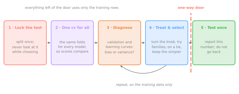
- Lock the test set before looking at anything: every decision made with it turns it into validation.
- One
cvfor every candidate, so that scores can be compared fold by fold. - Diagnose before tuning: the curves say whether the resource to spend is capacity, regularization or data.
- Treat and select with cross-validation, comparing families; on a tie within the noise, keep the simpler one. The winner's score is optimistic (section 8).
- Test once and report that number, without going back to stage 4 to "improve" it.
Advanced lab — select and test
The fundamental lab ended with three treated families: a regularized cubic Ridge, a tree with 10-district leaves and a k-NN with \(k = 10\). This part puts them in a single search, measures how reliable the ranking is, and only then opens the test set. Continue in the same notebook, in the same session: the steps below use pre, cv, rmse and candidates from steps 1 to 6.
How to do this lab in class (about 30 min, in pairs)
- Continue in the Colab notebook, from step 7. If the session dropped, first run the cells of steps 1 to 6 (Runtime → Run before).
- As in the fundamental lab: Predict before running, compare with this page, and try the Simulations before opening the solution.
- Suggested pace: step 7 and the first simulation in 12 min (the search takes about 20 seconds); step 8 in 8 min; step 9 and the second simulation in 10 min.
Step 7 — one search over the three families
Predict. A single search puts Ridge, k-NN and the tree side by side. Do you expect the winner to beat the best configuration of another family by more or by less than the fold-to-fold swing of their difference, about US$ 2,000?
from sklearn.model_selection import GridSearchCV
from sklearn.pipeline import Pipeline

pipe = Pipeline([('pre', pre), ('poly', PolynomialFeatures()), ('scale', StandardScaler()),
                 ('model', Ridge())])
param_grid = [
    {'model': [Ridge()], 'poly__degree': [1, 2, 3], 'model__alpha': [1, 10, 100, 1000]},
    {'model': [KNeighborsRegressor()], 'poly': ['passthrough'], 'scale': ['passthrough'],
     'model__n_neighbors': [5, 10, 20], 'model__weights': ['uniform', 'distance']},
    {'model': [DecisionTreeRegressor(random_state=42)], 'poly': ['passthrough'],
     'scale': ['passthrough'], 'model__min_samples_leaf': [5, 10, 20, 40]},
]
search = GridSearchCV(pipe, param_grid, cv=cv, scoring='neg_root_mean_squared_error', n_jobs=-1)
search.fit(X_train, y_train)


def describe(params):
    name = type(params['model']).__name__
    knobs = ', '.join(f"{k.split('__')[-1]}={v}" for k, v in params.items() if k != 'model'
                      and v != 'passthrough')
    return f"{name}({knobs})"


res = pd.DataFrame(search.cv_results_).sort_values('rank_test_score')
print(len(res), 'configurations ·', len(res) * cv.get_n_splits(), 'fits')
for _, row in res.head(6).iterrows():
    print(f"{row['rank_test_score']:2d}  {abs(row['mean_test_score']):6.0f} ± {row['std_test_score']:5.0f}"
          f"  {describe(row['params'])}")
22 configurations · 110 fits
 1   57473 ±  2381  Ridge(alpha=100, degree=3)
 2   57510 ±  2955  Ridge(alpha=10, degree=3)
 3   57796 ±  1534  DecisionTreeRegressor(min_samples_leaf=10)
 4   58079 ±  1214  DecisionTreeRegressor(min_samples_leaf=20)
 5   58517 ±  1084  KNeighborsRegressor(n_neighbors=10, weights=distance)
 6   59100 ±  1053  KNeighborsRegressor(n_neighbors=20, weights=distance)
Steps 3 to 6 were diagnosis; this is selection. One GridSearchCV holds the three families: the model slot takes a Ridge, a k-NN or a tree, and 'passthrough' disables the polynomial and scaling steps for the families that do not use them. 22 configurations, 110 fits, the same five folds as every earlier step.
The ranking has a clear message, and it is not "Ridge wins". The top three, 57,473, 57,510 and 57,796, come from two different families and lie within $323 of each other. The rule of the cross-validation lesson (compare fold by fold) compares a mean difference with the spread of the per-fold differences: for the winning Ridge and the best tree, a mean difference of $324 against a standard deviation of the differences of $1,943 (simulation below). That is a tie: the data cannot separate a regularized cubic Ridge from a tree with 10-district leaves. GridSearchCV returns rank 1 because it must return something. One difference is visible, though: the Ridge's fold standard deviation (2,381) is larger than the tree's (1,534), a trace of the erratic fold seen in step 6.
Simulation: the tie, fold by fold. Step 7 said the winning Ridge and the best tree are tied. Check it with the per-fold numbers: cv_results_ keeps every configuration's score on each of the five folds (split0_test_score, …). On how many folds is the Ridge ahead, and by how much?
Solution
res7 = pd.DataFrame(search.cv_results_)
i_ridge = res7['rank_test_score'].idxmin()
i_tree = res7[[type(p['model']).__name__ == 'DecisionTreeRegressor' for p in res7['params']]]['mean_test_score'].idxmax()
folds = pd.DataFrame({describe(res7.loc[i, 'params']): [abs(res7.loc[i, f'split{k}_test_score']) for k in range(5)]
                      for i in (i_ridge, i_tree)})
folds['tree - ridge'] = folds.iloc[:, 1] - folds.iloc[:, 0]
print(folds.round(0).astype(int).to_string())
d = folds['tree - ridge']
print(f"difference: mean {d.mean():.0f} · std {d.std(ddof=0):.0f} · ridge ahead in {(d > 0).sum()} of 5 folds")
   Ridge(alpha=100, degree=3)  DecisionTreeRegressor(min_samples_leaf=10)  tree - ridge
0                       55775                                       57848          2073
1                       60561                                       57664         -2896
2                       54694                                       57201          2507
3                       56265                                       55772          -493
4                       60068                                       60496           428
difference: mean 324 · std 1943 · ridge ahead in 3 of 5 folds
The Ridge is ahead on 3 folds and the tree on 2; the mean difference, US$ 324, is a sixth of the standard deviation of the differences (US$ 1,943). By the rule of the validation lesson, that is a tie: the sign of the difference flips from one fold to the next. Notice also that the two families fail in different ways: fold 1 is the Ridge's worst (60,561) and an ordinary fold for the tree. The hard folds are not the same for the two families, which suggests that averaging their predictions could err less than either one: the idea behind the ensemble lessons.
Step 8 — regression to the mean: re-measure the leaders
Predict. Validating the same 22 configurations on different folds, do the top three keep their order? And the order of the whole ranking, from best to worst?
search_new = GridSearchCV(pipe, param_grid, cv=KFold(n_splits=5, shuffle=True, random_state=7),
                          scoring='neg_root_mean_squared_error', n_jobs=-1).fit(X_train, y_train)
old = np.abs(search.cv_results_['mean_test_score'])
new = np.abs(search_new.cv_results_['mean_test_score'])
print('old rank  new rank    old RMSE  new RMSE')
for i in np.argsort(old)[:5]:
    print(f"{search.cv_results_['rank_test_score'][i]:8d} {search_new.cv_results_['rank_test_score'][i]:9d}"
          f" {old[i]:11.0f} {new[i]:9.0f}   {describe(search.cv_results_['params'][i])}")
print(f"old RMSE of all {len(old)} configurations: from {old.min():.0f} to {old.max():.0f}")
print(f"correlation between the two runs, all {len(old)} configurations: {np.corrcoef(old, new)[0, 1]:.3f}")
old rank  new rank    old RMSE  new RMSE
       1         2       57473     57232   Ridge(alpha=100, degree=3)
       2         1       57510     56498   Ridge(alpha=10, degree=3)
       3         4       57796     58385   DecisionTreeRegressor(min_samples_leaf=10)
       4         3       58079     58197   DecisionTreeRegressor(min_samples_leaf=20)
       5         6       58517     58693   KNeighborsRegressor(n_neighbors=10, weights=distance)
old RMSE of all 22 configurations: from 57473 to 68593
correlation between the two runs, all 22 configurations: 0.989
The same 22 configurations, cross-validated again with folds shuffled differently (random_state=7). Across all of them the two runs agree closely (correlation 0.989): the configurations differ a lot from each other (from $57,473 to $68,593), so most of their spread is "ability", and the reliability of the ranking as a whole is high.
Among the leaders it is another story. Rank 1 and rank 2 swap places, so do ranks 3 and 4, and individual scores move by up to $1,012 (57,510 → 56,498), three times the $323 that separated the top three. In the language of the regression-to-the-mean section, the spread of ability among the leaders is nearly zero, so their order is almost pure luck of the folds. What the reshuffle cannot show is whether the leaders are inflated: both runs use the same rows, so the luck of which districts were collected is the same in both, and the winner was chosen on them. Only data that played no part in the choice can show it, and step 9 does. The lesson from this step is narrower: a ranking inside the noise band is not a finding.
Step 9 — the one and only test
Predict. Will the winner's test RMSE land above, below or close to the US$ 57,473 of cross-validation? What difference would be a reason for concern?
from sklearn.metrics import mean_absolute_error, root_mean_squared_error

final = search.best_estimator_                        # already refit on all of X_train
pred = final.predict(X_test)
print(describe(search.best_params_))
print(f"CV RMSE (selection): {abs(search.best_score_):.0f}")
print(f"test RMSE (once):    {root_mean_squared_error(y_test, pred):.0f}")
print(f"test MAE:            {mean_absolute_error(y_test, pred):.0f}")
The winner meets the 4,128 locked-away districts, once: RMSE $56,790, against a cross-validated $57,473 that was used to select it. The difference, $683, is well inside one fold standard deviation (2,381): consistent with an honest estimate, and with a small winner's curse (about 13,000 training rows per fold, 22 candidates). The tie of step 7 means the tree with 10-district leaves would very likely have landed in the same place. The typical error is large: a mean absolute error of $39,278, on districts whose median value is around $180,000 (step 1).
Where does the remaining error live? The learning curves of step 4 were drawn for the untreated models (the winner's own curve is the first exercise below), so they only suggest an answer: the plain linear model had run out of what a hyperplane can learn, which the polynomial terms partly fixed, and the tree family was variance-limited, which is exactly what averaging many trees attacks: Random Forest and Gradient Boosting will return to this dataset's kind of problem. What you must not do now is go back to step 7 and try more settings until the test RMSE improves: the test set would become a validation set, and $56,790 would stop meaning anything.
Simulation: how precise is the test score? A single test score is also a noisy measurement: another 4,128 districts would give another number. Estimate that noise without touching new data: resample the test pairs (true value, prediction) with replacement 1,000 times and recompute the RMSE of each resample. Does the CV's US$ 57,473 fall inside the range?
Solution
boot = np.random.default_rng(0)
yt, pt = y_test.to_numpy(), pred
scores = []
for _ in range(1000):
    idx = boot.integers(0, len(yt), len(yt))           # one resample of the test districts
    scores.append(root_mean_squared_error(yt[idx], pt[idx]))
lo, hi = np.percentile(scores, [2.5, 97.5])
print(f"test RMSE {root_mean_squared_error(yt, pt):.0f} · 95% of resamples between {lo:.0f} and {hi:.0f} "
      f"(width {hi - lo:.0f})")
print(f"CV RMSE of the winner: {abs(search.best_score_):.0f}")
test RMSE 56790 · 95% of resamples between 54501 and 59002 (width 4501)
CV RMSE of the winner: 57473
95% of the resamples fall between US$ 54,501 and US$ 59,002: the test score means "about 57 thousand, give or take 2 thousand". The CV estimate, 57,473, sits well inside the range, so the US$ 683 difference between CV and test is evidence of nothing. This does not license testing the other two candidates to see which does better: the test score is only valid for the model chosen before looking.
To close the lesson. In one sentence each: (1) why does the score of a grid search's winner tend to drop when measured again? (2) How do you decide between two candidates whose mean difference is smaller than the spread of their per-fold differences? (3) Why does no model family win on every problem?
Your turn (advanced)
At home, with more time:
- Is the winner out of options? Draw the learning curve of the winning pipeline (
search.best_estimator_) as in step 4. Is it on the bias side or the variance side now, and would more districts help it? - Random instead of grid. Replace the grid of step 7 by
RandomizedSearchCVwithn_iter=20,loguniform(1, 1e4)foralphaandrandint(3, 60)forn_neighborsandmin_samples_leaf(fromscipy.stats). Does it find a configuration within one fold standard deviation of the grid's winner, with fewer fits? - Grade the procedure. Wrap
searchincross_val_score(search, X_train, y_train, cv=KFold(5, shuffle=True, random_state=1), scoring='neg_root_mean_squared_error')(nested CV). Compare the result withsearch.best_score_and with the test RMSE of step 9. - The right reliability. In the regression-to-the-mean simulation of section 8, what reliability \(r\) would make the top 10% keep half of their lead? Find the luck standard deviation that gives it, and check it with the code.
- A fifth family. Add
SVC(kernel='linear')with a grid overCto theparam_gridof section 9. On which datasets of the no-free-lunch table does it tie with the logistic regression, and why would you expect that?
References
- Geman, S.; Bienenstock, E.; Doursat, R. "Neural Networks and the Bias/Variance Dilemma." Neural Computation 4, no. 1 (1992): 1–58 — the paper that made the decomposition the standard lens on overfitting. DOI
- Hastie, T.; Tibshirani, R.; Friedman, J. The Elements of Statistical Learning, 2nd ed. Springer (2009), ch. 7 "Model Assessment and Selection" — the bias–variance decomposition, the effective number of parameters, cross-validation. free PDF
- Galton, F. "Regression toward Mediocrity in Hereditary Stature." Journal of the Anthropological Institute 15 (1886): 246–263 — regression to the mean, and the origin of the word. PDF (galton.org)
- Wolpert, D. H. "The Lack of A Priori Distinctions Between Learning Algorithms." Neural Computation 8, no. 7 (1996): 1341–1390 — the no-free-lunch theorems for supervised learning. DOI
- Stone, M. "Cross-Validatory Choice and Assessment of Statistical Predictions." JRSS B 36 (1974). DOI
- Bergstra, J.; Bengio, Y. "Random Search for Hyper-Parameter Optimization." JMLR 13 (2012). full text
- Pace, R. K.; Barry, R. "Sparse Spatial Autoregressions." Statistics & Probability Letters 33, no. 3 (1997): 291–297 — the California housing data used in the lab. DOI
Quiz
The quiz covers the fundamental approach.