The path of this part
- A common scalethe effective number of parameters
- Regression to the meanwhy the winner's score falls when measured again
- Compare familiesone search over all families, no free lunch, Occam's razor
- The whole workflowfive steps, a one-way door before the test, then the lab
A common scale: effective parameters
For models whose prediction is a weighted sum of the training labels: add up the weight each point gives to its own label.
\(n\): training points · \(p\): columns · \(k\): neighbors in k-nearest neighbors (k-NN) · \(\alpha\): the Ridge penalty.
| model | effective parameters | with \(n = 30\) |
|---|---|---|
| least squares, \(p\) columns | \(p\) | |
| k-NN | \(n / k\) | \(k = 30\): 1 · \(k = 3\): 10 · \(k = 1\): 30 |
| Ridge | falls from \(p\) toward 1 (the unpenalized intercept) as \(\alpha\) grows | continuous |
Regression to the mean
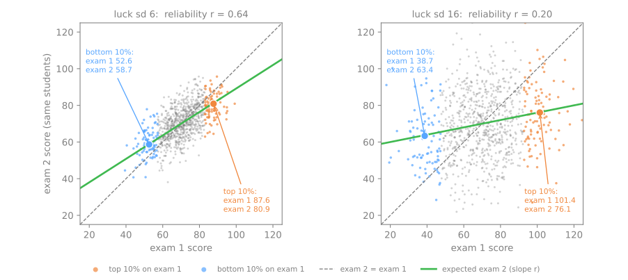
Score = ability (standard deviation, sd, 8) + luck of the day (its sd in the first column). Reliability: \(r = \frac{\sigma^2_\text{ability}}{\sigma^2_\text{ability} + \sigma^2_\text{luck}} = \frac{8^2}{8^2 + \text{luck}^2}\).
Predict. The top 10% on exam 1: do they keep their score on exam 2? And when luck grows?
| luck sd | \(r\) | exam 1 | exam 2 |
|---|---|---|---|
| 2 | 0.94 | 84.4 | 83.5 |
| 6 | 0.64 | 87.6 | 80.9 |
| 16 | 0.20 | 101.4 | 76.1 |
In model selection
- A configuration is a student; its future performance is the ability; its cross-validation (CV) score is an exam with luck (the folds, the sample).
- Near the top of a grid, configurations barely differ (little ability) while the CV noise stays the same: low reliability.
- More candidates → a more extreme winner → a luckier one. On pure noise, the best of 100 fell from 61.2% to 50.9%.
The family as a hyperparameter
pipe = Pipeline([('scale', StandardScaler()), ('model', LogisticRegression())])
param_grid = [                                     # a list of grids: one per family
    {'model': [LogisticRegression(max_iter=5000)], 'model__C': np.logspace(-3, 3, 7)},
    {'model': [KNeighborsClassifier()], 'model__n_neighbors': [1, 3, 5, 9, 15, 25, 51]},
    {'model': [SVC()], 'model__C': [0.1, 1, 10, 100], 'model__gamma': ['scale', 0.01, 0.1]},
    {'model': [DecisionTreeClassifier(random_state=0)], 'scale': ['passthrough'],
     'model__max_depth': [1, 2, 3, 4, 6, 8, 12, None]},
]
Radar returns: 34 configurations, 4 families, one search. Support vector machine (SVM) 0.946 · tree 0.897 · logistic 0.883 · k-NN 0.866.
model slot takes different estimators; 'passthrough' switches a step off. The same cv for all of them: they can be compared fold by fold.No free lunch
| dataset | logistic | k-NN | SVM | tree |
|---|---|---|---|---|
| ionosphere (real) | 0.883 | 0.866 | 0.946 | 0.897 |
| breast cancer (real) | 0.979 | 0.965 | 0.979 | 0.930 |
| credit-g (real) | 0.761 | 0.735 | 0.760 | 0.719 |
| linear, 40-d | 0.820 | 0.710 | 0.805 | 0.725 |
| two moons | 0.853 | 0.900 | 0.895 | 0.887 |
| axis-aligned rule | 0.640 | 0.636 | 0.686 | 0.938 |
What each family bets on
Logistic regression
the boundary is a hyperplane
k-NN
nearby points share labels
SVM with a radial basis function (RBF) kernel
the boundary is smooth
Tree
a few thresholds on a few features
Occam's razor, operationalized
- Breast cancer: logistic and SVM, both 0.979. Credit-g: 0.761 against 0.760.
- On a tie within the noise, keep the simpler one: 31 numbers and a dot product, against a set of support vectors and a kernel.
- Why? A more flexible model has noisier CV scores, so its narrow win is more likely selection luck; the simpler one also depends less on the sample, holds up better when the data change and is cheaper to run and explain.
The whole workflow
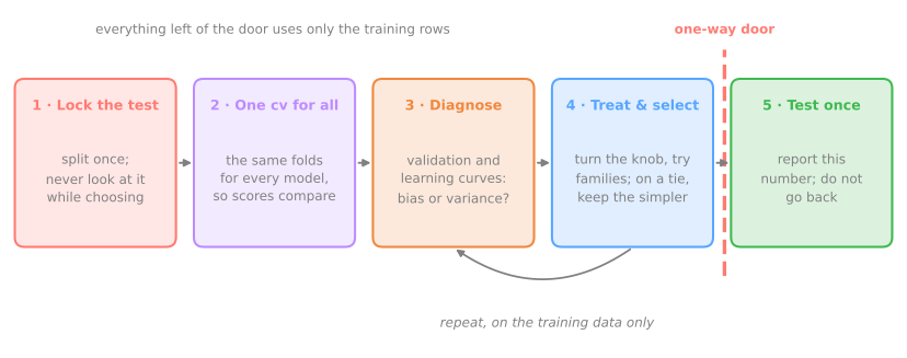
Select and test, steps 7 to 9
- Same notebook, same session: the steps use
pre,cv,rmseandcandidatesfrom steps 1 to 6. - One search with Ridge, k-NN and the tree; reshuffle the folds to see how much of the ranking is luck; open the test set once.
- Notebook on Colab (in Portuguese), from step 7.
- Simulations: the tie, fold by fold (step 7) and how precise is the test score? (step 9).
Pace: step 7 and the first simulation in 12 min; step 8 in 8 min; step 9 and the second simulation in 10 min.