The path of this part
- Two ways to be wrongmany fits of one truth: underfitting and overfitting
- Split the errorbias² + variance + noise, measured
- Diagnose with curvesvalidation curve, learning curve, the diagnosis
- Turn the knobeach family's complexity knob, then the lab: diagnose and treat
A worked example, by hand, at \(x = 0.25\)
Five training sets; each one fits a polynomial and predicts at \(x = 0.25\), where the truth is \(f(0.25) = 1\). \(\hat f_i\): the prediction from set \(i\); \(\overline{\hat f} = \tfrac{1}{5}\sum_i \hat f_i\): their average.
| training set \(i\) | 1 | 2 | 3 | 4 | 5 |
|---|---|---|---|---|---|
| degree 1 | 0.24 | 0.57 | 0.60 | 0.39 | 0.43 |
| degree 3 | 1.09 | 1.05 | 0.97 | 1.18 | 1.01 |
Predict. Which degree is right on average? Which one's five answers spread more?
- Bias \(= \overline{\hat f} - f(0.25)\). Degree 1: \(\overline{\hat f} = 0.446\), bias \(-0.554\), bias² 0.307. Degree 3: \(\overline{\hat f} = 1.060\), bias² 0.0036.
- Variance \(= \tfrac{1}{5}\sum_i \big(\hat f_i - \overline{\hat f}\big)^2\). Degree 1: 0.017. Degree 3: 0.0052.
Two ways to be wrong
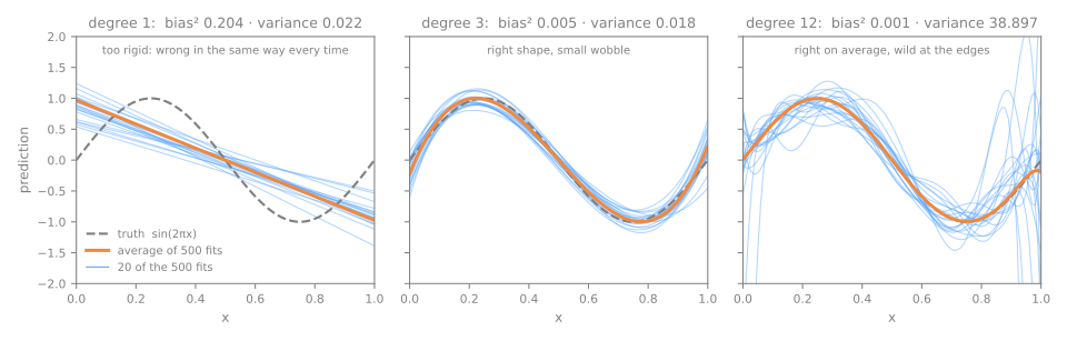
Truth: \(\sin(2\pi x)\). Each curve is a polynomial fitted to a different 30-point training set.
The dartboard: bias and variance
The decomposition
At a fixed \(x\): the truth \(f(x)\); a new observation \(y = f(x) + \varepsilon\), noise \(\varepsilon\) with mean 0 and variance \(\sigma^2\); the prediction \(\hat f(x)\), random because it depends on the training set; \(\mathbb{E}\): the average over training sets and noise.
\[ \mathbb{E}\big[(y - \hat f(x))^2\big] = \underbrace{\big(f(x) - \mathbb{E}[\hat f(x)]\big)^2}_{\text{bias}^2} + \underbrace{\mathbb{E}\big[(\hat f(x) - \mathbb{E}[\hat f(x)])^2\big]}_{\text{variance}} + \underbrace{\sigma^2}_{\text{noise}} \]- \(y - \hat f = (f - \hat f) + \varepsilon\); the new \(\varepsilon\) has mean 0 and is independent of the training set, so the cross term vanishes: \(\mathbb{E}[(y - \hat f)^2] = \mathbb{E}[(f - \hat f)^2] + \sigma^2\).
- For any random \(Z\): \(\mathbb{E}[Z^2] = (\mathbb{E}[Z])^2 + \operatorname{Var}(Z)\). With \(Z = f - \hat f\): bias² + variance.
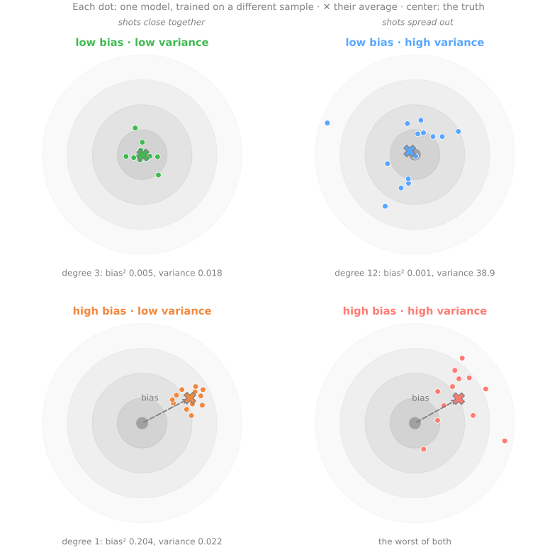
Bias: the family's best attempt is wrong on average (a line cannot follow a sine). Variance: the price of listening to the sample. Noise: the part of \(y\) that does not depend on \(x\); here \(\sigma^2 = 0.3^2 = 0.09\), and nobody goes below it.
Measured with 500 training sets
Predict. 500 training sets of 30 points per degree. At which degree is the test mean squared error (MSE) lowest? And what happens to the variance at degree 12?
| degree | bias² | variance | noise | sum | measured test MSE |
|---|---|---|---|---|---|
| 0 | 0.495 | 0.020 | 0.09 | 0.605 | 0.603 |
| 1 | 0.204 | 0.022 | 0.09 | 0.316 | 0.314 |
| 3 | 0.005 | 0.018 | 0.09 | 0.113 | 0.112 |
| 5 | 0.000 | 0.045 | 0.09 | 0.135 | 0.135 |
| 7 | 0.001 | 0.635 | 0.09 | 0.726 | 0.723 |
| 12 | 0.001 | 38.897 | 0.09 | 38.987 | 38.985 |
- The columns add up by construction (the decomposition is an identity): the sum matches the error measured on new data up to the fresh noise (difference ≤ 0.004).
- Bias falls to zero; variance rises slowly, then violently. The bottom of the U: degree 3. The large variances are orders of magnitude: a handful of the 500 samples produce most of them.
Three families, the same U
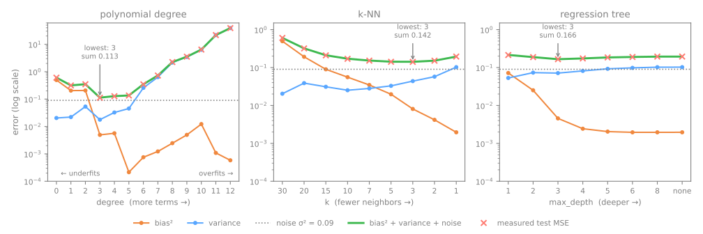
- k-nearest neighbors (k-NN) with \(k = 30\) (every point) is the degree-0 polynomial; in k-NN, small \(k\) is the complex model.
- 1-NN copies one noisy label: variance ≈ \(\sigma^2\) (the noise variance, 0.09), test error ≈ \(2\sigma^2\) (measured: 0.195).
Simulator: underfit ↔ overfit, live
Predict. Slide the degree from 0 (pure bias) to 12 (pure variance). Which error only falls, and which one turns back up?
Validation curve: the U without knowing the truth
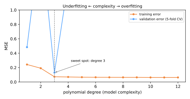
- Training only falls: 0.267 → 0.046. Choosing by it always picks the most complex model.
- On the left: both high and close — bias.
- On the right: training falls, validation climbs to 1.748 — variance.
- Bottom at degree 3 (0.114): the same as the 500-sample simulation.
Learning curve: is more data worth it?
Predict. More and more training points: does the error of degree 1 keep falling? And that of degree 9?
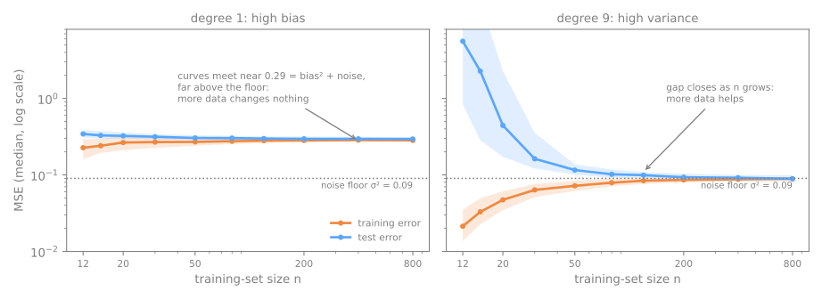
- Median of 300 training sets per size.
- Degree 1: training and test meet near 0.29 and stay there. More data does not help.
- Degree 9: test error 5.6 with 12 points, at the noise floor by about 200. With its coefficients fixed, data closes the gap.
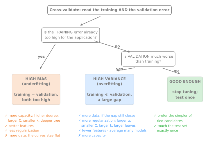
The diagnosis
Every family has a knob
Predict. To make each model more complex, which way do you turn degree, alpha, C, n_neighbors, max_depth and min_samples_leaf?
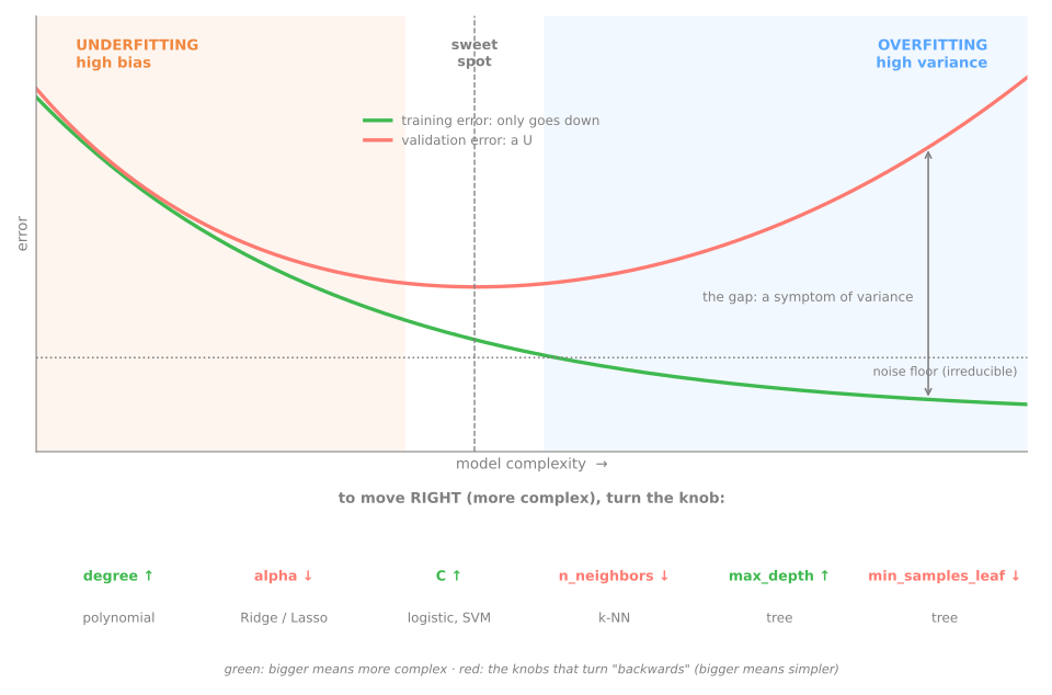
The ones that turn "backwards" are the confusing ones: larger alpha, k and min_samples_leaf make the model simpler.
Summary
- Test error = bias² + variance + noise. The noise is a floor.
- Bias: training ≈ validation, both high. Variance: training ≪ validation.
- A validation curve varies complexity; a learning curve varies the data.
- For a model of fixed capacity, more data cures variance and not bias; more capacity only cures bias.
- Every model has a complexity knob, and some turn backwards.
| symptom | diagnosis | what to do |
|---|---|---|
| training ≈ validation, both high | bias | more capacity, better features |
| training ≪ validation, gap closing | variance | more data, more regularization |
House prices: diagnose and treat, steps 1 to 6
- California housing: 20,640 districts, 9 features, target = median house value.
- Three families (linear, k-NN, tree): which suffers from bias and which from variance? Would more data help? Which knob to turn?
- Notebook on Colab (in Portuguese): nothing to download. Save a copy to your Drive.
- At every step, answer the Predict before running.
- Simulations: variance, up close (step 3) and alpha as a continuous knob (step 6).
Pace: steps 1 to 3 and the first simulation in 15 min; steps 4 to 6 and the second in 25 min.