Neural Networks
A neural network is built from a part you already know well. The logistic regression of the logistic regression lesson computes a weighted sum of the features, adds a bias and squashes the result with a sigmoid: that is one artificial neuron. A neural network connects many of them in layers, so that the outputs of one layer become the features of the next, and trains all their weights together by gradient descent.
This lesson builds that idea in small steps, each one measured: the single neuron and Rosenblatt's perceptron (with a simulator), the XOR problem that no single neuron can solve, a two-layer network that solves it with weights chosen by hand, why the activation function must be nonlinear, the forward pass as matrix products, backpropagation worked out number by number on a 2-2-1 network, and finally scikit-learn's MLPClassifier in practice, including an honest comparison with the gradient boosting of the previous lesson on tabular data. It ends with a step-by-step backpropagation simulator. The full story (convolutional networks, transformers, PyTorch) belongs to the Deep Learning course; here the goal is to understand what a network computes and how it learns. Every number quoted comes from the code blocks or from the figure scripts next to this page.
The lesson follows one pipeline in five stages, drawn below: 1. one neuron, logistic regression read as a neuron and the perceptron; 2. hidden layers, XOR and why the activation must be nonlinear; 3. forward pass, what a network computes, as matrix products; 4. backpropagation, how every weight learns from the error; 5. in practice, training with scikit-learn and when a network is worth it. Each stage links to its section, and in the slides a strip at the bottom shows which stage you are in.
- One neuronlogistic regression as a neuron; the perceptron
- Hidden layersXOR, a hidden layer, nonlinear activations
- Forward passone matrix product per layer; counting parameters
- Backpropagationchain rule, six steps, a non-convex loss
- In practicescaling, width, weight decay; tabular data
Slides
Click the slides and use the ← → arrows to navigate; F goes full screen and Esc shows every slide. Open the slides in a new tab
From logistic regression to a neuron
Stage 1. An artificial neuron takes inputs \(x_1, \dots, x_d\), computes a pre-activation \(z\) (a weighted sum plus a bias) and passes it through an activation function \(\varphi\):
With \(\varphi = \sigma\), the sigmoid \(\sigma(z) = 1/(1 + e^{-z})\), this is exactly logistic regression: \(a\) is the predicted probability of the positive class. A numeric example with \(w = (2, -1)\), \(b = 0.5\) and the input \(x = (1, 2)\): \(z = 2 \cdot 1 - 1 \cdot 2 + 0.5 = 0.5\) and \(a = \sigma(0.5) = 0.622\).
Everything in this lesson changes one of two things: the activation \(\varphi\) (a step, a sigmoid, a ReLU) or the wiring (one neuron, or layers of them feeding each other). The first historical choice was a step.
The perceptron
The update rule
Frank Rosenblatt's perceptron (1958) is a neuron whose activation is a step: it answers \(+1\) if \(z > 0\) and \(-1\) otherwise, with labels \(y \in \{-1, +1\}\) as in the SVM lesson. It was built as a machine, the Mark I Perceptron, with photocells as inputs and motor-driven potentiometers as weights. Its learning rule needs no calculus. Visit the training points one at a time; if point \(i\) is on the wrong side of the boundary, or exactly on it (\(y_i z_i \le 0\)), move the weights toward it:
if it is on the correct side, change nothing. Why this helps: after the update, the same point's score becomes
that is, the signed score of the misclassified point grows by \(\eta(\lVert x_i \rVert^2 + 1) > 0\): the boundary tilts and shifts toward classifying it correctly. One update may not be enough, and it may break another point, which is why the procedure loops over the data in epochs (full passes) until one epoch makes no mistake.
Three updates by hand
Six points, three of each class, and a start at \(w = (0, 0)\), \(b = 0\), \(\eta = 1\):
| point | \(x_1\) | \(x_2\) | \(y\) |
|---|---|---|---|
| A | 4 | 2 | +1 |
| B | 0 | 2 | −1 |
| C | 1 | 3 | −1 |
| D | 2 | 4 | −1 |
| E | 3 | 0 | +1 |
| F | 3 | 1 | +1 |
By hand, epoch 1.
- A: \(z = 0\), so \(y z = 0 \le 0\), a mistake (every point is "on the line" when \(w = 0\)). Update: \(w = (0, 0) + (+1)(4, 2) = (4, 2)\), \(b = 0 + 1 = 1\).
- B: \(z = 4 \cdot 0 + 2 \cdot 2 + 1 = 5\), but \(y = -1\): \(y z = -5\), a mistake. Update: \(w = (4, 2) - (0, 2) = (4, 0)\), \(b = 1 - 1 = 0\).
- C: \(z = 4 \cdot 1 + 0 \cdot 3 + 0 = 4\), \(y = -1\): a mistake. Update: \(w = (4, 0) - (1, 3) = (3, -3)\), \(b = -1\).
- D, E, F: \(z = 3 \cdot 2 - 3 \cdot 4 - 1 = -7\), \(z = 9 - 0 - 1 = 8\), \(z = 9 - 3 - 1 = 5\), all on the correct side. No change.
Epoch 2 visits all six points without a mistake, so the perceptron stops with the boundary \(3x_1 - 3x_2 - 1 = 0\), the line \(x_2 = x_1 - \tfrac{1}{3}\). The code follows the same steps:
import numpy as np
import pandas as pd

X = np.array([[4, 2], [0, 2], [1, 3], [2, 4], [3, 0], [3, 1]])
y = np.array([+1, -1, -1, -1, +1, +1])


def perceptron(X, y, eta=1.0, epochs=20, trace=False):
    """Rosenblatt's rule: visit the points in order, update only on mistakes."""
    w, b = np.zeros(X.shape[1]), 0.0
    history = []                                   # (mistakes, w, b) at the end of each epoch
    for epoch in range(1, epochs + 1):
        mistakes = 0
        for i in range(len(X)):
            z = w @ X[i] + b
            mistake = y[i] * z <= 0                # wrong side, or on the line
            if mistake:
                w, b = w + eta * y[i] * X[i], b + eta * y[i]
                mistakes += 1
            if trace and epoch == 1:
                print(f"x = ({X[i][0]:g}, {X[i][1]:g})  y = {y[i]:+d}  z = {z:+g}  y·z = {y[i] * z + 0.0:+g}  "   # + 0.0: print -0 as 0
                      + (f"mistake -> w = ({w[0]:g}, {w[1]:g}), b = {b:g}" if mistake else "correct"))
        history.append((mistakes, w.copy(), b))
        if mistakes == 0:
            break
    return w, b, history


w, b, history = perceptron(X, y, trace=True)
print("mistakes per epoch:", [m for m, _, _ in history])
print(f"final w = ({w[0]:g}, {w[1]:g}), b = {b:g}")
x = (4, 2)  y = +1  z = +0  y·z = +0  mistake -> w = (4, 2), b = 1
x = (0, 2)  y = -1  z = +5  y·z = -5  mistake -> w = (4, 0), b = 0
x = (1, 3)  y = -1  z = +4  y·z = -4  mistake -> w = (3, -3), b = -1
x = (2, 4)  y = -1  z = -7  y·z = +7  correct
x = (3, 0)  y = +1  z = +8  y·z = +8  correct
x = (3, 1)  y = +1  z = +5  y·z = +5  correct
mistakes per epoch: [3, 0]
final w = (3, -3), b = -1
The library implements the same rule. scikit-learn's Perceptron, with a constant step eta0=1 and the points visited in their original order (shuffle=False), lands on the same weights; and because the start is \(w = 0\), the step size only rescales them:
from sklearn.linear_model import Perceptron

skl = Perceptron(eta0=1.0, shuffle=False, tol=None, max_iter=20).fit(X, y)
print("scikit-learn:", skl.coef_[0], skl.intercept_[0])
w_small, b_small, _ = perceptron(X, y, eta=0.1)
print("eta = 0.1:   ", w_small.round(2), round(b_small, 2), "-> the same line, scaled by 0.1")
The four states of the boundary: no line at the start, then one line after each update (figure script):
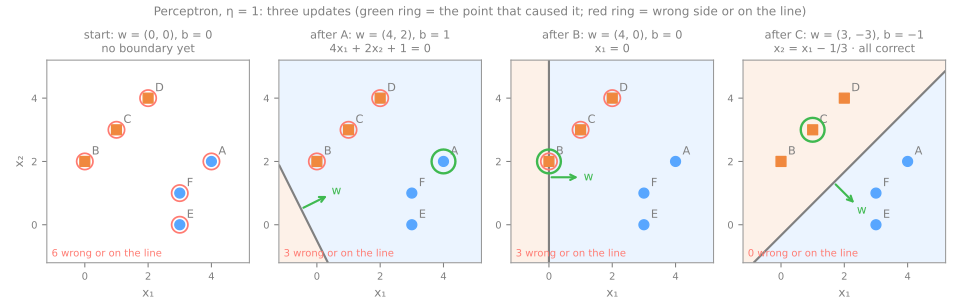
Notice what the update does geometrically. The vector \(w\) is perpendicular to the boundary and points to the \(+1\) side. A mistake on a \(-1\) point (B, C) subtracts that point from \(w\), rotating the \(+1\) side away from it; a mistake on a \(+1\) point adds it.
Convergence. If a line separates the two classes with some margin \(\gamma > 0\) and every point lies within distance \(R\) of the origin (counting the bias as an extra input fixed at 1), the perceptron makes at most \((R / \gamma)^2\) mistakes, whatever the order of the points (Novikoff, 1962). It stops at some separating line, not the best one; choosing the widest street is what the SVM adds. And if no line separates the classes, the theorem promises nothing, as the next section shows.
Try it: the perceptron simulator
The simulator runs the same rule. Step visits one point and shows the arithmetic: the score \(z\), the test \(y z \le 0\) and, on a mistake, the update with its numbers. Whole epoch runs to the end of the current pass, and Play animates. The first preset is the six-point example above; the second draws a new random separable dataset at each click; the third is XOR, the subject of the next section: watch the mistakes per epoch never reach zero.
XOR: why one line is not enough
Stage 2. The exclusive-or has four points: \((0, 1)\) and \((1, 0)\) are \(+1\), \((0, 0)\) and \((1, 1)\) are \(-1\). No line puts the two diagonals on different sides. The algebra is short: a separating line would need
- \((0,0)\) negative: \(b < 0\);
- \((0,1)\) and \((1,0)\) positive: \(w_2 + b > 0\) and \(w_1 + b > 0\);
- \((1,1)\) negative: \(w_1 + w_2 + b < 0\).
Adding the two middle inequalities gives \(w_1 + w_2 + 2b > 0\), so \(w_1 + w_2 + b > -b > 0\), which contradicts the last one. The perceptron keeps trying anyway:
X_xor = np.array([[0, 0], [0, 1], [1, 0], [1, 1]])
y_xor = np.array([-1, +1, +1, -1])

w, b, history = perceptron(X_xor, y_xor, epochs=8, trace=True)
print("mistakes per epoch:", [m for m, _, _ in history])
print("weights at the end of every epoch:", {f"w = ({w_e[0]:g}, {w_e[1]:g}), b = {b_e:g}" for _, w_e, b_e in history})
x = (0, 0)  y = -1  z = +0  y·z = +0  mistake -> w = (0, 0), b = -1
x = (0, 1)  y = +1  z = -1  y·z = -1  mistake -> w = (0, 1), b = 0
x = (1, 0)  y = +1  z = +0  y·z = +0  mistake -> w = (1, 1), b = 1
x = (1, 1)  y = -1  z = +3  y·z = -3  mistake -> w = (0, 0), b = 0
mistakes per epoch: [4, 4, 4, 4, 4, 4, 4, 4]
weights at the end of every epoch: {'w = (0, 0), b = 0'}
Every visit is a mistake, and the four updates of an epoch add up to exactly zero: \(\sum_i y_i x_i = -(0,0) + (0,1) + (1,0) - (1,1) = (0,0)\) and \(\sum_i y_i = 0\). So after each epoch the weights are back at \(w = (0, 0)\), \(b = 0\), and the same four updates repeat forever. From another start or in another order the path is different, but it never ends, because no epoch can be free of mistakes.
This is the observation that Minsky and Papert made famous in their book Perceptrons (1969): a single-layer perceptron cannot compute XOR, nor, more generally, any function that depends on a feature combination no line can express. The book was read as a verdict on neural networks as a whole, and funding moved elsewhere for over a decade, part of what the introduction calls the first AI winter.
The same wall stops logistic regression, which is also a single neuron. Measured on a noisy XOR, 400 points scattered around the four corners, with 5-fold cross-validation:
from sklearn.linear_model import LogisticRegression
from sklearn.model_selection import StratifiedKFold, cross_val_score

rng = np.random.default_rng(0)
corners = rng.integers(0, 2, size=(400, 2))              # each point starts at a corner of the square
X_nx = corners + rng.normal(0, 0.2, size=(400, 2))       # and is blurred by noise
y_nx = corners[:, 0] ^ corners[:, 1]                     # label: XOR of the corner's coordinates
cv = StratifiedKFold(n_splits=5, shuffle=True, random_state=0)

print("class balance:", np.bincount(y_nx))
print(f"logistic regression, CV accuracy: {cross_val_score(LogisticRegression(), X_nx, y_nx, cv=cv).mean():.3f}")
p = LogisticRegression().fit(X_nx, y_nx).predict_proba(X_nx)[:, 1]
print(f"fitted on all 400 points, P(class 1) goes only from {p.min():.2f} to {p.max():.2f}")
class balance: [205 195]
logistic regression, CV accuracy: 0.485
fitted on all 400 points, P(class 1) goes only from 0.37 to 0.61
The classes are balanced (205 and 195 points), so guessing is right about half the time, and logistic regression does no better: 0.485. A line could do better than chance (cutting off one corner gets three of the four corners right), but the log loss prefers to hedge: fitted on all 400 points, the predicted probability of class 1 stays between 0.37 and 0.61 everywhere. One neuron has nothing better to offer.
A hidden layer solves XOR
The way out is to stop asking one neuron to do everything. XOR is "\(x_1\) OR \(x_2\), but NOT both", and each of those pieces is linearly separable. So use two neurons to compute the pieces, and a third to combine them:
- hidden neuron \(h_1\) fires when \(x_1 + x_2 - 0.5 > 0\): that is OR;
- hidden neuron \(h_2\) fires when \(x_1 + x_2 - 1.5 > 0\): that is AND;
- the output fires when \(h_1 - h_2 - 0.5 > 0\): "OR and not AND", which is XOR.
Every weight here was chosen by hand. The table, for the four inputs:
step = lambda z: (z > 0).astype(int)

X4 = np.array([[0, 0], [0, 1], [1, 0], [1, 1]])
W1 = np.array([[1, 1],        # h1: x1 + x2 - 0.5 > 0  (OR)
               [1, 1]])       # h2: x1 + x2 - 1.5 > 0  (AND)
b1 = np.array([-0.5, -1.5])
w2, b2 = np.array([1, -1]), -0.5                    # output: h1 - h2 - 0.5 > 0

Z1 = X4 @ W1.T + b1                                 # hidden pre-activations, one row per input
H = step(Z1)                                        # hidden activations
z_out = H @ w2 + b2
print(pd.DataFrame({'x1': X4[:, 0], 'x2': X4[:, 1], 'z1': Z1[:, 0], 'h1 (OR)': H[:, 0],
                    'z2': Z1[:, 1], 'h2 (AND)': H[:, 1], 'z_out': z_out,
                    'output': step(z_out), 'XOR': X4[:, 0] ^ X4[:, 1]}).to_string(index=False))
 x1  x2   z1  h1 (OR)   z2  h2 (AND)  z_out  output  XOR
  0   0 -0.5        0 -1.5         0   -0.5       0    0
  0   1  0.5        1 -0.5         0    0.5       1    1
  1   0  0.5        1 -0.5         0    0.5       1    1
  1   1  1.5        1  0.5         1   -0.5       0    0
Check the row \((1, 1)\) with a calculator: \(z_1 = 1 + 1 - 0.5 = 1.5\), so \(h_1 = 1\); \(z_2 = 1 + 1 - 1.5 = 0.5\), so \(h_2 = 1\); \(z_{\text{out}} = 1 - 1 - 0.5 = -0.5\), so the output is 0. The network computes XOR exactly.
What happened is easier to see than to say (figure script):
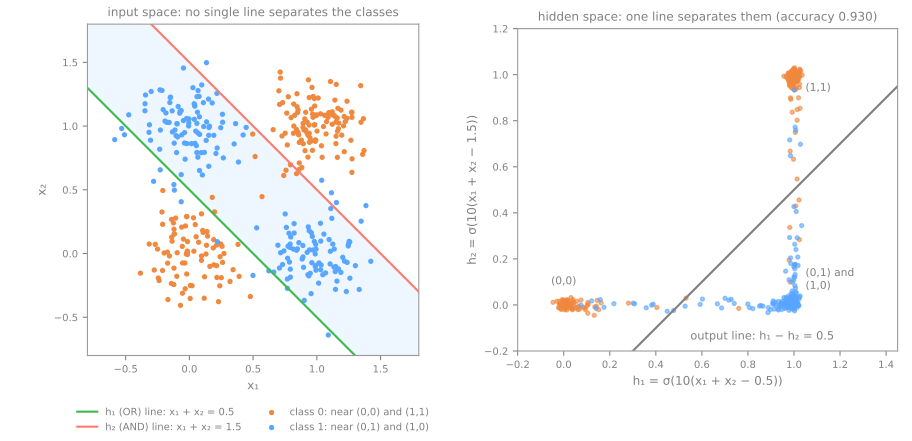
On the left, each hidden neuron draws one line in the input space, and class 1 is the band between the two lines, something no single line can describe. On the right is the same data seen through the hidden layer, \((h_1, h_2)\) instead of \((x_1, x_2)\) (with the sigmoid version of the network, below, so that the noisy points do not all collapse onto exactly three corners). In that new space, \((0,0)\) stays at \((0,0)\), \((1,1)\) goes to \((1,1)\), and both class-1 corners land on \((1, 0)\). Now one line separates the classes, and the output neuron only has to draw it.
That is the central idea of the lesson: the hidden layer computes new features in which the problem becomes linearly separable, and the output layer is a linear classifier on those features. You have done this by hand before, adding \(x^2\) columns as polynomial features or letting the SVM kernel do it implicitly. A network learns its features, from the data, by gradient descent.
There is one obstacle. Gradient descent needs derivatives, and the step function has derivative 0 everywhere (and none at 0): a small change of a weight never changes the output, so the gradient says nothing. The fix is to replace the step by a smooth function with the same shape. With the sigmoid and every weight multiplied by 10, the same network outputs probabilities:
sigmoid = lambda z: 1 / (1 + np.exp(-z))

H_soft = sigmoid(10 * (X4 @ W1.T + b1))
p = sigmoid(10 * (H_soft @ w2 + b2))
print(pd.DataFrame({'x1': X4[:, 0], 'x2': X4[:, 1], 'h1': H_soft[:, 0].round(3),
                    'h2': H_soft[:, 1].round(3), 'P(XOR = 1)': p.round(3)}).to_string(index=False))
 x1  x2    h1    h2  P(XOR = 1)
  0   0 0.007 0.000       0.007
  0   1 0.993 0.007       0.992
  1   0 0.993 0.007       0.992
  1   1 1.000 0.993       0.007
The two class-0 inputs get probability 0.007 and the two class-1 inputs 0.992: the same network, now differentiable. Multiplying the weights by 10 makes each sigmoid steep, close to a step; smaller weights would give softer probabilities. This is the kind of network a gradient-based trainer can find by itself from random weights, which is what MLPClassifier does in the next sections.
Activation functions
Sigmoid, tanh and ReLU
Three activations cover almost all practice:
| activation | \(\varphi(z)\) | range | derivative \(\varphi'(z)\) | largest derivative |
|---|---|---|---|---|
| sigmoid | \(1 / (1 + e^{-z})\) | \((0, 1)\) | \(\varphi(z)\,(1 - \varphi(z))\) | 0.25, at \(z = 0\) |
| tanh | \((e^{z} - e^{-z}) / (e^{z} + e^{-z})\) | \((-1, 1)\) | \(1 - \varphi(z)^2\) | 1, at \(z = 0\) |
| ReLU | \(\max(0, z)\) | \([0, \infty)\) | 0 if \(z < 0\), 1 if \(z > 0\) | 1, for every \(z > 0\) |
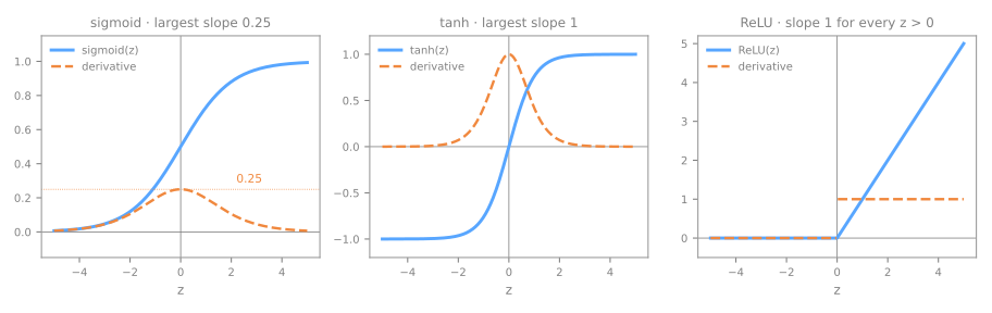
The derivative column is what matters for training, because backpropagation (below) multiplies one activation derivative per layer. With sigmoids, each layer multiplies the gradient by at most 0.25; through 10 layers that is at most \(0.25^{10} \approx 10^{-6}\), and the first layers barely learn. This vanishing gradient is why the ReLU (Nair & Hinton, 2010; Glorot, Bordes & Bengio, 2011) became the default for hidden layers: its slope is exactly 1 wherever the neuron is active. It is scikit-learn's default too (activation='relu'). Sigmoid remains the natural choice for the output of a binary classifier, because it produces a probability, exactly as in logistic regression; for \(k\) classes the output is a softmax.
Without a nonlinearity, layers collapse
Why not skip the activation and stack plain linear layers? Because a linear function of a linear function is linear. Two layers \(W_2 (W_1 x + b_1) + b_2\) equal one layer with weights \(W_2 W_1\) and bias \(W_2 b_1 + b_2\). Numerically, with random weights (3 hidden units):
rng = np.random.default_rng(0)
W1r, b1r = rng.normal(size=(3, 2)), rng.normal(size=3)       # layer 1: 2 inputs -> 3 units
W2r, b2r = rng.normal(size=(1, 3)), rng.normal(size=1)       # layer 2: 3 units -> 1 output
x_new = np.array([1.0, -2.0])

two_linear_layers = W2r @ (W1r @ x_new + b1r) + b2r
W_merged, b_merged = W2r @ W1r, W2r @ b1r + b2r
print("two linear layers:", two_linear_layers.round(4))
print("one merged layer: ", (W_merged @ x_new + b_merged).round(4), "with W =", W_merged.round(3))
print("with a ReLU between them:", (W2r @ np.maximum(0, W1r @ x_new + b1r) + b2r).round(4))
two linear layers: [-5.4084]
one merged layer:  [-5.4084] with W = [[-0.58   0.117]]
with a ReLU between them: [-5.3273]
The two linear layers and the merged single layer print the same number, −5.4084, and they would for any input: the three hidden units added nothing, and the whole 2 → 3 → 1 network is the linear model \(-0.58\,x_1 + 0.117\,x_2 + b\). Put a ReLU between the layers and the output changes (−5.3273 here), because the network can no longer be rewritten as a single matrix.
The same thing, measured on the noisy XOR: an MLPClassifier with 8 hidden units and activation='identity' (no nonlinearity) against the same network with ReLU, on the same folds as logistic regression:
from sklearn.neural_network import MLPClassifier
from sklearn.pipeline import make_pipeline
from sklearn.preprocessing import StandardScaler

for act in ['identity', 'relu']:
    net = make_pipeline(StandardScaler(),
                        MLPClassifier(hidden_layer_sizes=(8,), activation=act, max_iter=2000, random_state=0))
    print(f"8 hidden units, activation={act:8s}: CV accuracy {cross_val_score(net, X_nx, y_nx, cv=cv).mean():.3f}")
8 hidden units, activation=identity: CV accuracy 0.510
8 hidden units, activation=relu    : CV accuracy 0.983
Without an activation, the 8-unit network is a linear model in disguise and scores 0.510, the same chance level as logistic regression (0.485). With ReLU it reaches 0.983. The units, the solver and the data are identical; only the nonlinearity changed.
The forward pass as matrix products
One layer is one matrix product
Stage 3. Write the weights of a layer as a matrix, one row per neuron. For the 2-2-1 network below:
For a whole batch of \(n\) rows at once, stack the inputs as the rows of \(X\) and the same computation is \(H = \sigma(X W^\top + b^h)\): one matrix product and one elementwise function per layer. This is the forward pass, and it is why neural networks run so well on GPUs, which are machines for multiplying matrices.
A 2-2-1 network, by hand
The network below is the one used in the Deep Learning course and in the simulator at the end of this page: two inputs, two sigmoid hidden units, one sigmoid output, one training example \(x = (0.5, 0.8)\) with target \(y = 0\), and these starting weights:
| from → to | weight | from → to | weight |
|---|---|---|---|
| \(x_1 \to h_1\) | \(w_{11} = 0.2\) | \(h_1 \to \hat y\) | \(v_{11} = 0.3\) |
| \(x_2 \to h_1\) | \(w_{12} = 0.4\) | \(h_2 \to \hat y\) | \(v_{12} = 0.5\) |
| \(x_1 \to h_2\) | \(w_{21} = 0.6\) | bias \(\to \hat y\) | \(b^{y}_1 = 0.4\) |
| \(x_2 \to h_2\) | \(w_{22} = 0.8\) | ||
| bias \(\to h_1\) | \(b^{h}_1 = 0.1\) | ||
| bias \(\to h_2\) | \(b^{h}_2 = 0.2\) |
By hand: \(z_1 = 0.2 \cdot 0.5 + 0.4 \cdot 0.8 + 0.1 = 0.52\) and \(z_2 = 0.6 \cdot 0.5 + 0.8 \cdot 0.8 + 0.2 = 1.14\); \(h_1 = \sigma(0.52)\) and \(h_2 = \sigma(1.14)\); then \(u = 0.3 h_1 + 0.5 h_2 + 0.4\) and \(\hat y = \sigma(u)\). To keep the numbers identical to the Deep Learning course, this example measures the error with the squared loss \(L = (\hat y - y)^2\):
x = np.array([0.5, 0.8])
y_true = 0.0
W = np.array([[0.2, 0.4],       # row i = the weights into hidden unit h_i
              [0.6, 0.8]])
b_h = np.array([0.1, 0.2])
v = np.array([0.3, 0.5])        # weights into the output
b_y = 0.4

z = W @ x + b_h                 # hidden pre-activations
h = sigmoid(z)                  # hidden activations
u = v @ h + b_y                 # output pre-activation
y_hat = sigmoid(u)              # output
L = (y_hat - y_true) ** 2       # squared loss
print("z =", z.round(3), " h =", h.round(3))
print(f"u = {u:.3f}  y_hat = {y_hat:.3f}  L = {L:.4f}")
The hidden pre-activations are \(z = (0.52, 1.14)\), the hidden activations \(h = (0.627, 0.758)\), the output pre-activation \(u = 0.3 \cdot 0.627 + 0.5 \cdot 0.758 + 0.4 = 0.967\) and the prediction \(\hat y = \sigma(0.967) = 0.725\). The target is 0, so the network is quite wrong: \(L = 0.725^2 = 0.5249\).
scikit-learn computes the same thing. Load these weights into an MLPClassifier with sigmoid hidden units (activation='logistic'); its coefs_ hold one matrix per layer, stored as (inputs × units), the transpose of our \(W\):
import warnings
from sklearn.exceptions import ConvergenceWarning

warnings.filterwarnings('ignore', category=ConvergenceWarning)
net = MLPClassifier(hidden_layer_sizes=(2,), activation='logistic', max_iter=1).fit([[0, 0], [1, 1]], [0, 1])
net.coefs_ = [W.T, v.reshape(2, 1)]              # our weights replace the ones it started with
net.intercepts_ = [b_h, np.array([b_y])]
print("scikit-learn P(y = 1 | x) =", net.predict_proba([x])[0, 1].round(4))
Counting parameters
A layer with \(n_\text{in}\) inputs and \(n_\text{out}\) units has \(n_\text{in} \cdot n_\text{out}\) weights and \(n_\text{out}\) biases, \((n_\text{in} + 1) \cdot n_\text{out}\) parameters in all. For 8 × 8 images of digits (64 pixels, 10 classes):
def n_params(sizes):
    return sum((n_in + 1) * n_out for n_in, n_out in zip(sizes[:-1], sizes[1:]))


for sizes in [(2, 2, 1), (64, 10), (64, 32, 10), (64, 256, 10), (64, 64, 64, 10)]:
    print(f"{' -> '.join(map(str, sizes)):22s} {n_params(sizes):6,d} parameters")
2 -> 2 -> 1                 9 parameters
64 -> 10                  650 parameters
64 -> 32 -> 10          2,410 parameters
64 -> 256 -> 10        19,210 parameters
64 -> 64 -> 64 -> 10    8,970 parameters
The 2-2-1 network has 9 parameters (6 in the first layer, 3 in the second): the ones in the table above. Softmax regression on 64 pixels has \(65 \cdot 10 = 650\). A hidden layer of 32 units takes the count to \(65 \cdot 32 + 33 \cdot 10 = 2{,}410\), and 256 units to 19,210, more parameters than there are images in the whole digits dataset (1,797). Two hidden layers of 64 units have fewer parameters (8,970) than one of 256: the count grows with the product of neighboring widths. With that many parameters per example, regularization (below) is not optional.
Training: backpropagation
The loss and the chain rule
Stage 4. Training means choosing all the weights to minimize a loss over the training set. scikit-learn's MLPClassifier minimizes the same cross-entropy as logistic regression, plus an L2 penalty on the weights, \(\tfrac{\alpha}{2} \lVert W \rVert^2\), the same penalty as Ridge; in the neural-network literature it is called weight decay, and in scikit-learn it is the parameter alpha. Gradient descent needs \(\partial L / \partial w\) for every weight \(w\). The output layer's weights are easy, but a weight of the first layer influences the loss only through everything after it:
The chain rule multiplies the local derivatives along that path. Backpropagation (Rumelhart, Hinton & Williams, 1986) is the chain rule organized so that nothing is computed twice: start at the loss, compute the derivative with respect to each layer's pre-activation (called its delta, \(\delta\)), and pass it backwards one layer at a time. Every weight's gradient is then "the delta of the unit it feeds × the value that came into it".
For the 2-2-1 network, with the squared loss, the six steps are:
- loss gradient: \(\partial L / \partial \hat y = 2(\hat y - y)\);
- output delta: \(\delta_y = \partial L / \partial u = 2(\hat y - y) \cdot \hat y (1 - \hat y)\), because \(\sigma'(u) = \hat y(1 - \hat y)\);
- output weights: \(\partial L / \partial v_{1j} = \delta_y \, h_j\) and \(\partial L / \partial b^y_1 = \delta_y\);
- hidden deltas: \(\delta_{h_j} = \delta_y \, v_{1j} \cdot h_j (1 - h_j)\), the output delta sent back along the weight \(v_{1j}\), times the local sigmoid slope;
- hidden weights: \(\partial L / \partial w_{jk} = \delta_{h_j} \, x_k\) and \(\partial L / \partial b^h_j = \delta_{h_j}\);
- update every parameter: \(p \leftarrow p - \eta \, \partial L / \partial p\).
The six steps, with numbers
dL_dyhat = 2 * (y_hat - y_true)                  # 1. loss gradient
delta_y = dL_dyhat * y_hat * (1 - y_hat)         # 2. output delta, dL/du
grad_v = delta_y * h                             # 3. output weights
grad_b_y = delta_y
delta_h = delta_y * v * h * (1 - h)              # 4. hidden deltas, dL/dz
grad_W = np.outer(delta_h, x)                    # 5. hidden weights: delta of the unit × its input
grad_b_h = delta_h

print(f"1. dL/dy_hat = 2({y_hat:.3f} - {y_true:.0f}) = {dL_dyhat:.3f}")
print(f"2. delta_y   = {dL_dyhat:.3f} · {y_hat:.3f}(1 - {y_hat:.3f}) = {delta_y:.4f}")
print(f"3. dL/dv     = {grad_v.round(4)}   dL/db_y = {grad_b_y:.4f}")
print(f"4. delta_h   = {delta_h.round(4)}")
print(f"5. dL/dW     = {grad_W.round(4).tolist()}   dL/db_h = {grad_b_h.round(4)}")
1. dL/dy_hat = 2(0.725 - 0) = 1.449
2. delta_y   = 1.449 · 0.725(1 - 0.725) = 0.2892
3. dL/dv     = [0.1814 0.2191]   dL/db_y = 0.2892
4. delta_h   = [0.0203 0.0266]
5. dL/dW     = [[0.0101, 0.0162], [0.0133, 0.0212]]   dL/db_h = [0.0203 0.0266]
Read the numbers from top to bottom:
- the loss gradient, 1.449: if \(\hat y\) rises a little, the loss rises about 1.449 times as much, so training must push \(\hat y\) down toward the target 0;
- the output delta, 0.289: the sigmoid's slope at the output is \(0.725 \times 0.275 = 0.199\), and \(1.449 \times 0.199 = 0.289\);
- the output weights: \(0.289 \times h\) gives 0.181 for \(v_{11}\) and 0.219 for \(v_{12}\), larger because \(h_2 = 0.758\) contributed more to the output;
- the hidden deltas, 0.0203 and 0.0266: about ten times smaller than the output delta, because on the way back each was multiplied by a weight below 1 (0.3 and 0.5) and by a sigmoid slope below 0.25 (\(0.627 \times 0.373 = 0.234\) for \(h_1\));
- the first-layer gradients, the hidden deltas times the inputs 0.5 and 0.8, range from 0.0101 to 0.0212: the smallest of all. That is the vanishing gradient of the activation section, in miniature.
Is that really the derivative? Check it the slow way: nudge each of the 9 parameters by \(\pm 10^{-6}\), recompute the loss, and take the difference quotient (a finite-difference check):
def loss(params):
    W_, b_h_, v_, b_y_ = params[:4].reshape(2, 2), params[4:6], params[6:8], params[8]
    return (sigmoid(v_ @ sigmoid(W_ @ x + b_h_) + b_y_) - y_true) ** 2


params = np.r_[W.ravel(), b_h, v, b_y]           # the 9 parameters in one vector
backprop = np.r_[grad_W.ravel(), grad_b_h, grad_v, grad_b_y]
eps = 1e-6
numeric = np.array([(loss(params + eps * e) - loss(params - eps * e)) / (2 * eps) for e in np.eye(9)])
print("largest difference, backprop vs finite differences:", f"{np.abs(numeric - backprop).max():.1e}")

eta = 0.5                                        # 6. one gradient step on all 9 parameters
new_params = params - eta * backprop
print(f"loss before: {loss(params):.4f} · after one step with eta = {eta}: {loss(new_params):.4f}")
largest difference, backprop vs finite differences: 1.3e-10
loss before: 0.5249 · after one step with eta = 0.5: 0.4405
Backpropagation and the finite differences agree to within \(10^{-10}\), the rounding error of the difference quotients: backpropagation is not an approximation but the exact derivative, computed efficiently. One gradient step with \(\eta = 0.5\) on all 9 parameters lowers the loss on this example from 0.5249 to 0.4405.
The finite-difference check needed 18 extra forward passes for 9 parameters; backpropagation got all 9 gradients from one backward pass, which costs about as much as the forward pass. For the 2,410 parameters of a 64-32-10 digit network that is one backward pass instead of 4,820 forward passes, and for modern networks with billions of parameters the ratio is what makes training possible at all.
A remark that links back to logistic regression: with the cross-entropy loss instead of the squared loss, steps 1 and 2 collapse into one, \(\delta_y = \hat y - y\) (here \(0.725\)), the same "prediction minus target" as in the gradient of logistic regression. Everything from step 3 on is unchanged.
Non-convex: the starting point matters
For logistic regression the loss is convex: one minimum, reached from any start. Composing layers breaks that. The same 2-hidden-unit network that solves XOR by hand, trained from 10 random initializations (the random_state), on the noisy XOR:
for units in [2, 8]:
    accs = [make_pipeline(StandardScaler(), MLPClassifier(hidden_layer_sizes=(units,), max_iter=5000,
                                                          random_state=seed)).fit(X_nx, y_nx).score(X_nx, y_nx)
            for seed in range(10)]
    print(f"{units} hidden units, training accuracy for seeds 0-9:", np.round(accs, 2))
2 hidden units, training accuracy for seeds 0-9: [0.76 0.66 0.74 0.94 0.94 0.94 0.94 0.94 0.74 0.66]
8 hidden units, training accuracy for seeds 0-9: [0.98 0.98 0.97 0.98 0.98 0.96 0.99 0.99 0.97 0.95]
With 2 hidden units, 5 of the 10 starts reach 0.94 training accuracy, about as good as the hand-built network (0.930 on these same points, computed in the figure script above). The other 5 stop at 0.66 to 0.76, stuck in a worse local minimum. With 8 units every start ends between 0.95 and 0.99: extra units give gradient descent more routes to a good solution, one reason practical networks are wider than the minimum that could work. In scikit-learn the start is set by random_state: fix it for reproducibility, and when a conclusion matters, check that it holds for a few seeds.
Optimizers and regularization
MLPClassifier offers three solvers. 'adam' (the default; Kingma & Ba, 2015) is mini-batch gradient descent (batches of 200 rows) with momentum and a per-parameter step size; it is the workhorse for large datasets. 'sgd' is plain mini-batch gradient descent, with optional momentum. 'lbfgs' uses the whole training set at every step and an approximation of the curvature; on small datasets (a few thousand rows) it usually converges faster and better.
Regularization, in the vocabulary you already have:
alpha, weight decay: the L2 penalty of Ridge, on every weight of every layer;early_stopping=True: hold out 10% of the training rows, track accuracy on them after each epoch, and stop when it has not improved for 10 epochs (n_iter_no_change), the same idea as early stopping in gradient boosting;- in deep-learning libraries there is also dropout (Srivastava et al., 2014), which switches off a random subset of units at each step so that no unit can rely on a specific other one; scikit-learn does not implement it.
Training in practice with scikit-learn
Scale the inputs
Stage 5. Gradient descent on a network suffers from features on different scales exactly as it did for linear models: the loss surface becomes a long narrow valley, and one learning rate cannot suit every direction. On the spambase dataset (4,601 e-mails, 57 numeric features: word and character frequencies, and lengths of runs of capital letters that go into the thousands):
from sklearn.datasets import fetch_openml

spam = fetch_openml(data_id=44, as_frame=True)                 # spambase (UCI)
X_sp, y_sp = spam.data, (spam.target == '1').astype(int)       # 1 = spam
print(X_sp.shape, f"spam share {y_sp.mean():.3f}",
      f"· feature std from {X_sp.std().min():.3f} to {X_sp.std().max():.0f}")

for name, model in [('raw inputs', MLPClassifier(max_iter=1000, random_state=0)),
                    ('StandardScaler first', make_pipeline(StandardScaler(),
                                                           MLPClassifier(max_iter=1000, random_state=0)))]:
    print(f"MLP, {name:20s}: CV accuracy {cross_val_score(model, X_sp, y_sp, cv=cv).mean():.3f}")
(4601, 57) spam share 0.394 · feature std from 0.076 to 606
MLP, raw inputs          : CV accuracy 0.927
MLP, StandardScaler first: CV accuracy 0.948
The feature standard deviations range from 0.076 to 606. On raw inputs the MLP reaches a CV accuracy of 0.927; with a StandardScaler in front, 0.948, two points more from one line of preprocessing. The scaler goes inside the pipeline, so that each fold fits it on its own training rows, as in the pipelines lesson. (Spambase has 394 exact duplicate e-mails, kept here; the decision-trees lesson explains why dropping them gives slightly lower, more honest scores.)
Width: how many hidden units?
hidden_layer_sizes=(h,) sets one hidden layer of \(h\) units; (h1, h2) sets two layers. More units mean more pieces the network can combine, so a more flexible boundary. On 300 points of two noisy half-moons, with the 'lbfgs' solver and almost no weight decay (alpha=1e-4):
from sklearn.datasets import make_moons
from sklearn.model_selection import cross_validate

X_m, y_m = make_moons(n_samples=300, noise=0.3, random_state=1)


def train_and_cv(units, alpha):
    net = make_pipeline(StandardScaler(), MLPClassifier(hidden_layer_sizes=(units,), solver='lbfgs',
                                                        alpha=alpha, max_iter=5000, random_state=0))
    r = cross_validate(net, X_m, y_m, cv=cv, return_train_score=True)
    return f"train {r['train_score'].mean():.3f} · CV {r['test_score'].mean():.3f}"


print(f"logistic regression:  CV {cross_val_score(LogisticRegression(), X_m, y_m, cv=cv).mean():.3f}")
for units in [1, 3, 10, 100]:
    print(f"{units:3d} hidden units: ", train_and_cv(units, alpha=1e-4))
logistic regression:  CV 0.830
  1 hidden units:  train 0.842 · CV 0.843
  3 hidden units:  train 0.897 · CV 0.873
 10 hidden units:  train 0.938 · CV 0.893
100 hidden units:  train 0.997 · CV 0.857
With 1 hidden unit the network is no better than logistic regression (CV 0.843 against 0.830): one unit draws one line. With 3 and 10 units the boundary bends and CV accuracy rises to 0.873 and 0.893. With 100 units the network fits the training folds almost perfectly (0.997) while CV accuracy falls back to 0.857: it now has enough units to wrap individual noisy points, the same overfitting you saw with deep decision trees and high polynomial degrees.
Weight decay: alpha
Keep the 100 units and raise alpha:
for alpha in [1e-4, 0.01, 0.1, 1, 10]:
    print(f"100 units, alpha = {alpha:<6g}:", train_and_cv(100, alpha))
100 units, alpha = 0.0001: train 0.997 · CV 0.857
100 units, alpha = 0.01  : train 0.993 · CV 0.880
100 units, alpha = 0.1   : train 0.939 · CV 0.903
100 units, alpha = 1     : train 0.914 · CV 0.917
100 units, alpha = 10    : train 0.837 · CV 0.830
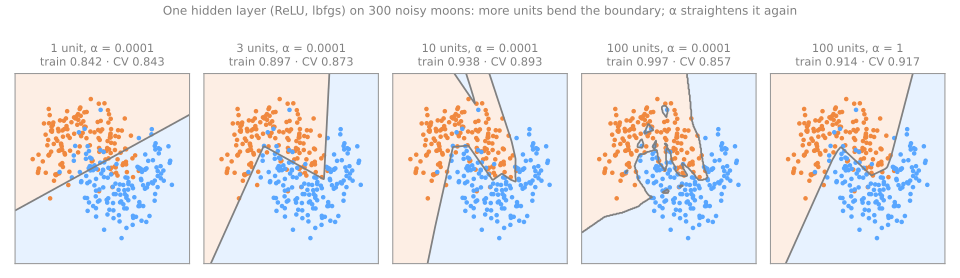
The table and the figure tell the story of Ridge again. With almost no penalty the 100 units overfit (training 0.997, CV 0.857). Raising alpha shrinks the weights, the boundary smooths out and the gap between training and CV closes: at alpha = 1, training is 0.914 and CV 0.917, the best setting on this page and better than 10 units without penalty (0.893). Too much penalty flattens the network back to a line: alpha = 10 gives 0.830, logistic regression's score. Notice also the shape of the boundaries: with ReLU units they are made of straight segments, with a bend wherever a unit switches on or off, which is easy to see in the 3- and 10-unit panels.
The practical recipe, then, is the one of every model in this course: choose a generous architecture, and tune alpha (and the width) with cross-validation. The lab does exactly that.
Why depth, and when to use a neural network
Depth
One hidden layer is already a universal approximator: with enough units it can approximate any continuous function on a bounded region as closely as desired (Cybenko, 1989; Hornik, 1991). The theorem guarantees existence, not that training finds the weights, nor that the number of units is reasonable. In practice, deep networks (many layers) reach the same accuracy with far fewer units, because each layer builds on the features of the previous one: in images, the first layers of a convolutional network respond to edges, the next ones to textures and parts, the last ones to whole objects. That hierarchy is why deep learning took over perception problems (images, audio, text) from 2012 on, when data and GPUs became plentiful (AlexNet).
Tabular data: an honest comparison
On a table of heterogeneous columns, the story is different. Same folds, same spambase data, four models:
from sklearn.ensemble import HistGradientBoostingClassifier

candidates = {
    'logistic': make_pipeline(StandardScaler(), LogisticRegression(max_iter=5000)),
    'MLP': make_pipeline(StandardScaler(), MLPClassifier(max_iter=1000, random_state=0)),
    'MLP early stop': make_pipeline(StandardScaler(),
                                    MLPClassifier(max_iter=1000, early_stopping=True, random_state=0)),
    'boosting': HistGradientBoostingClassifier(random_state=0),
}
folds = pd.DataFrame({name: cross_val_score(m, X_sp, y_sp, cv=cv) for name, m in candidates.items()})
print(pd.concat([folds, folds.agg(['mean', 'std'])]).round(3).to_string())
print("boosting - MLP, per fold:", (folds['boosting'] - folds['MLP']).round(3).tolist())
      logistic    MLP  MLP early stop  boosting
0        0.921  0.951           0.946     0.954
1        0.928  0.953           0.950     0.955
2        0.926  0.946           0.937     0.966
3        0.934  0.949           0.942     0.965
4        0.913  0.941           0.935     0.939
mean     0.924  0.948           0.942     0.956
std      0.008  0.005           0.006     0.011
boosting - MLP, per fold: [0.003, 0.002, 0.021, 0.016, -0.002]
On this table the ranking is gradient boosting 0.956 ± 0.011, MLP 0.948 ± 0.005, MLP with early stopping 0.942 ± 0.006, logistic regression 0.924 ± 0.008. Boosting beats the MLP in 4 of the 5 folds, but by little (from −0.002 to 0.021): an edge, not a knockout. And it got there with its defaults and no preprocessing, while the network needed a scaler, a choice of architecture, alpha and solver, and gains nothing from early stopping here.
This matches large benchmarks: on typical tabular datasets, tree ensembles remain as good as or better than neural networks, with less tuning and less compute (Shwartz-Ziv & Armon, 2022; Grinsztajn, Oyallon & Varoquaux, 2022). Trees split on one feature at a time, so they are insensitive to scale, ignore useless columns easily and handle irregular, step-like relations between a feature and the target; a network must learn all of that from smooth functions. On images the balance flips, as the lab shows on pixels.
| data | first choice |
|---|---|
| tables of heterogeneous columns | gradient boosting or a random forest |
| images, audio, video | convolutional networks, vision transformers |
| text | transformers, or embeddings + a linear model |
| few rows | linear models, k-NN, SVM |
Where to go next: the Deep Learning course
This lesson stops at the multi-layer perceptron. The companion course Artificial Neural Networks and Deep Learning continues from exactly here: its MLP lesson derives backpropagation in matrix form, and the course goes on to training deep networks (initialization, normalization, dropout), convolutional and recurrent networks, transformers and generative models, in PyTorch instead of scikit-learn.
Backpropagation, step by step: the simulator
The simulator replays the computation of the backpropagation section on the same 2-2-1 network. Step 1 is the forward pass, with every value kept on its node; steps 2 to 6 send the gradient backwards, from the loss to the first layer, one chain-rule link at a time; step 7 applies the update with \(\eta = 0.5\). The numbers are the ones printed by the code of that section. Use Next and Back, the dots, or the arrow keys.
Lab: a neural network on handwritten digits
The problem. The digits dataset that ships with scikit-learn holds 1,797 handwritten digits, scanned and reduced to 8 × 8 images with 17 gray levels (0 to 16), from the UCI "Optical Recognition of Handwritten Digits" collection. Each image becomes a row of 64 pixel values, and the task is to name the digit. Pixels are not a table of heterogeneous columns: every column is the same kind of measurement, and what matters is how neighboring pixels combine, the kind of structure a hidden layer can learn.
The workflow is the one from the validation lesson: lock a test set away, compare models on the same cross-validation folds, tune with GridSearchCV, and touch the test set once. Every output below is what the code prints. To run it yourself, download the lab notebook and open it in Jupyter or Colab (File → Upload notebook); it runs in about a minute.
Step 1 — load and look
import numpy as np
import pandas as pd
import matplotlib.pyplot as plt
from sklearn.datasets import load_digits

X, y = load_digits(return_X_y=True)          # 1,797 images of 8 × 8 pixels, one row of 64 values each
print(X.shape, "· pixel values from", X.min(), "to", X.max())
print("images per digit:", np.bincount(y))

fig, axes = plt.subplots(1, 10, figsize=(10, 1.4))
for digit, ax in enumerate(axes):
    ax.imshow(X[y == digit][0].reshape(8, 8), cmap='gray_r')
    ax.set_title(digit)
    ax.axis('off')
plt.show()
(1797, 64) · pixel values from 0.0 to 16.0
images per digit: [178 182 177 183 181 182 181 179 174 180]
1,797 images, 64 pixel columns with values from 0 to 16, and between 174 and 183 images per digit: the classes are balanced, so accuracy is a fair summary. The row of thumbnails shows how coarse 8 × 8 pixels are. All the columns are in the same unit, but the network is trained by gradient descent, so it gets a StandardScaler in its pipeline anyway.
Step 2 — lock the test set away
from sklearn.model_selection import train_test_split

X_train, X_test, y_train, y_test = train_test_split(
    X, y, test_size=0.25, stratify=y, random_state=42)
print(X_train.shape, X_test.shape)
1,347 images for development and 450 locked away until step 8, both with the same share of each digit thanks to stratify=y. On the test set each image is worth 0.22 points of accuracy (1/450).
Step 3 — a baseline and the folds everyone shares
from sklearn.dummy import DummyClassifier
from sklearn.model_selection import StratifiedKFold, cross_val_score

cv = StratifiedKFold(n_splits=5, shuffle=True, random_state=42)


def cv_summary(model):
    scores = cross_val_score(model, X_train, y_train, cv=cv)
    return f"{scores.mean():.3f} ± {scores.std():.3f}"


print("always the most frequent digit:", cv_summary(DummyClassifier(strategy='most_frequent')))
Always answering the most frequent digit is right 10.0% of the time, with no variation across folds because stratification gives every fold the same class shares. Every accuracy below must be read against 0.100. The cv object is created once and reused in every step, so all models are scored on the same five folds, and cv_summary reports the mean ± standard deviation over them.
Step 4 — three models on the same folds
from sklearn.ensemble import RandomForestClassifier
from sklearn.linear_model import LogisticRegression
from sklearn.neural_network import MLPClassifier
from sklearn.pipeline import make_pipeline
from sklearn.preprocessing import StandardScaler

models = {
    'logistic regression': make_pipeline(StandardScaler(), LogisticRegression(max_iter=2000)),
    'random forest, 300 trees': RandomForestClassifier(n_estimators=300, random_state=42, n_jobs=-1),
    'MLP, defaults (100 units)': make_pipeline(StandardScaler(), MLPClassifier(max_iter=1000, random_state=42)),
}
for name, model in models.items():
    print(f"{name:26s} {cv_summary(model)}")
logistic regression        0.966 ± 0.010
random forest, 300 trees   0.976 ± 0.009
MLP, defaults (100 units)  0.974 ± 0.010
All three are far above the 0.100 baseline. Logistic regression, a linear model on the raw pixels, already reaches 0.966; the random forest 0.976; the MLP with scikit-learn's defaults (one hidden layer of 100 ReLU units, alpha = 0.0001, the Adam solver) 0.974. That MLP has \((64 + 1) \cdot 100 + (100 + 1) \cdot 10 = 7{,}510\) parameters. The gaps between the three (0.002 to 0.010) are about the size of one fold standard deviation (0.009 to 0.010), so nothing is decided yet.
Step 5 — tune the width and alpha
from sklearn.model_selection import GridSearchCV

mlp = make_pipeline(StandardScaler(), MLPClassifier(max_iter=1000, random_state=42))
param_grid = {'mlpclassifier__hidden_layer_sizes': [(16,), (64,), (256,), (64, 64)],
              'mlpclassifier__alpha': [0.0001, 1, 10]}
grid = GridSearchCV(mlp, param_grid, cv=cv, n_jobs=-1).fit(X_train, y_train)

res = pd.DataFrame(grid.cv_results_)
res['layers'] = res['param_mlpclassifier__hidden_layer_sizes'].astype(str)
table = res.pivot(index='layers', columns='param_mlpclassifier__alpha', values='mean_test_score')
print(table.reindex(['(16,)', '(64,)', '(256,)', '(64, 64)']).round(3))
best_std = res.loc[grid.best_index_, 'std_test_score']
print(f"best: {grid.best_params_} · CV accuracy {grid.best_score_:.3f} ± {best_std:.3f}")
param_mlpclassifier__alpha  0.0001   1.0000   10.0000
layers
(16,)                         0.959    0.969    0.951
(64,)                         0.977    0.977    0.951
(256,)                        0.982    0.975    0.950
(64, 64)                      0.973    0.973    0.941
best: {'mlpclassifier__alpha': 0.0001, 'mlpclassifier__hidden_layer_sizes': (256,)} · CV accuracy 0.982 ± 0.003
Read the table by rows and by columns:
- width helps, up to a point: 16 units are too few (0.959 without penalty), 64 and 256 reach 0.977 and 0.982;
alpha = 10hurts every architecture (0.941 to 0.951): the penalty squeezes the weights until the network underfits.alpha = 1helps the smallest network (0.969 against 0.959) and slightly hurts the largest (0.975 against 0.982);- a second hidden layer does not help here: (64, 64) scores 0.973, below a single layer of 64 (0.977). Depth pays off on perceptual data at a much larger scale than 1,347 images of 8 × 8 pixels.
The winner, 256 units with alpha = 0.0001, scores 0.982 ± 0.003; the runners-up at 0.977 are less than two fold standard deviations behind. As in the validation lesson, a good choice rather than a proven optimum.
Step 6 — the loss curve and early stopping
best = grid.best_estimator_                        # the winner, refit on all of X_train
net = best[-1]
print(f"no early stopping: {net.n_iter_} epochs · final training loss {net.loss_curve_[-1]:.4f}")

settings = {k.split('__')[1]: v for k, v in grid.best_params_.items()}
early = make_pipeline(StandardScaler(), MLPClassifier(**settings, early_stopping=True, max_iter=1000,
                                                      random_state=42)).fit(X_train, y_train)
net_es = early[-1]
print(f"early stopping:    {net_es.n_iter_} epochs · best accuracy on its 10% validation rows "
      f"{net_es.best_validation_score_:.3f}")
print("CV accuracy with early stopping:", cv_summary(early))

fig, ax = plt.subplots(figsize=(7, 3.2))
ax.plot(net.loss_curve_, label='training loss, no early stopping')
ax.plot(net_es.loss_curve_, label='training loss, early stopping')
ax.set_xlabel('epoch')
ax.set_ylabel('training loss')
ax.set_yscale('log')
ax2 = ax.twinx()
ax2.plot(net_es.validation_scores_, color='green', label='validation accuracy (early stopping)')
ax2.set_ylabel('validation accuracy')
fig.legend(loc='center right')
plt.show()
no early stopping: 105 epochs · final training loss 0.0039
early stopping:    31 epochs · best accuracy on its 10% validation rows 0.978
CV accuracy with early stopping: 0.961 ± 0.008
Without early stopping, Adam ran 105 epochs (passes over the 1,347 training images), until the loss stopped improving, and ended at a training loss of 0.0039: the network fits its training images almost perfectly and confidently. With early_stopping=True, scikit-learn set aside 10% of the training rows, stopped after 31 epochs because accuracy on them had not improved since epoch 20, and reached 0.978 on them (figure script):
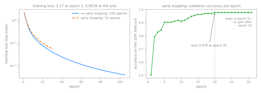
Its cross-validated accuracy, however, is 0.961 ± 0.008, below the winner's 0.982. On a dataset this small, giving up 10% of the training rows and stopping early costs more than the overfitting it prevents; the penalty alpha, chosen by cross-validation, is the better regularizer here. Early stopping earns its place on large datasets, where each epoch is expensive and there are rows to spare.
Step 7 — is the MLP really better? Same folds, fold by fold
def fold_scores(g):                                # the 5 fold scores of a grid's winner
    return np.array([g.cv_results_[f'split{k}_test_score'][g.best_index_] for k in range(5)])


lr_grid = GridSearchCV(models['logistic regression'],
                       {'logisticregression__C': [0.01, 0.1, 1, 10, 100]}, cv=cv).fit(X_train, y_train)
print("logistic regression, best C:", lr_grid.best_params_['logisticregression__C'])
folds = pd.DataFrame({'MLP': fold_scores(grid),
                      'logistic': fold_scores(lr_grid),
                      'forest': cross_val_score(models['random forest, 300 trees'], X_train, y_train, cv=cv)})
folds['MLP - logistic'] = folds['MLP'] - folds['logistic']
folds['MLP - forest'] = folds['MLP'] - folds['forest']
print(pd.concat([folds, folds.agg(['mean', 'std'])]).round(3).to_string())
logistic regression, best C: 10
        MLP  logistic  forest  MLP - logistic  MLP - forest
0     0.978     0.956   0.974           0.022         0.004
1     0.985     0.981   0.974           0.004         0.011
2     0.981     0.963   0.989           0.019        -0.007
3     0.981     0.959   0.963           0.022         0.019
4     0.985     0.978   0.981           0.007         0.004
mean  0.982     0.967   0.976           0.015         0.006
std   0.003     0.012   0.010           0.009         0.010
Tuned over C, logistic regression settles at C = 10 and 0.967. Then, fold by fold:
- the MLP beats the tuned logistic regression in all five folds, by 0.004 to 0.022, mean 0.015 ± 0.009: the features learned by the hidden layer are worth about 1.5 points of accuracy on pixels;
- against the random forest it wins 4 folds of 5 and loses one (−0.007), mean 0.006 ± 0.010: a difference smaller than its own standard deviation, so a tie.
The caveats of the validation lesson apply: the MLP's column is the best of 12 configurations, so it is slightly optimistic, while the forest ran with its defaults. On pixels the network is at least as good as a strong tree ensemble; on the spambase table of the lesson, boosting was ahead.
Step 8 — the one and only test
from sklearn.metrics import accuracy_score, confusion_matrix

pred = best.predict(X_test)
print(f"test accuracy {accuracy_score(y_test, pred):.3f} · {(pred != y_test).sum()} errors in {len(y_test)} images")
cm = confusion_matrix(y_test, pred)
errors = cm - np.diag(np.diag(cm))                 # keep only the mistakes
true_d, pred_d = np.unravel_index(errors.argmax(), errors.shape)
print(f"most frequent mistake: true {true_d}, predicted {pred_d} ({errors[true_d, pred_d]} times)")
print("errors per true digit:", errors.sum(axis=1))
test accuracy 0.982 · 8 errors in 450 images
most frequent mistake: true 8, predicted 1 (3 times)
errors per true digit: [1 1 0 0 0 1 1 0 4 0]
Once, at the end, the tuned MLP meets the 450 test images: accuracy 0.982, 8 errors, exactly the cross-validated estimate (0.982 ± 0.003). Half of the errors (4 of 8) are true 8s, three of them read as 1s, while digits 2, 3, 4, 7 and 9 have no test errors at all. With 8 × 8 pixels there is little room to tell a narrow 8 from a 1.
Your turn
- Depth. Add
(128, 64)and(256, 128)to the grid of step 5. Does a second hidden layer beat the best single layer by more than one fold standard deviation? Count the parameters of each winner withn_paramsfrom the lesson. - Gradient boosting on pixels. Evaluate
HistGradientBoostingClassifier(random_state=42)withcv_summary(it takes longer than the others). On spambase it beat the MLP; what happens on pixels? Put its fold scores next to the MLP's as in step 7. - Solver and activation. Refit the winner with
solver='lbfgs'and then withactivation='tanh', on the same folds. Which setting changes the CV accuracy more than its standard deviation? - Look at the mistakes. Plot the misclassified test images (
X_test[pred != y_test], reshaped to 8 × 8) with their true and predicted labels. Would you have read them correctly?
Class materials
Videos
- But what is a neural network? — 3Blue1Brown, Deep Learning chapter 1
- Backpropagation calculus — 3Blue1Brown, Deep Learning chapter 4
Further reading
- ANN-DL — Multi-Layer Perceptron — the same 2-2-1 example, in depth
- TensorFlow Playground — train a small network in the browser and watch its hidden units
- scikit-learn User Guide — Neural network models (supervised)
References
- Rosenblatt, F. "The Perceptron: A Probabilistic Model for Information Storage and Organization in the Brain." Psychological Review 65, no. 6 (1958): 386–408. DOI
- Novikoff, A. B. J. "On Convergence Proofs on Perceptrons." Proceedings of the Symposium on the Mathematical Theory of Automata 12 (1962): 615–622 — the mistake bound \((R/\gamma)^2\).
- Minsky, M.; Papert, S. Perceptrons: An Introduction to Computational Geometry. MIT Press (1969) — the XOR limitation of single-layer perceptrons.
- Rumelhart, D. E.; Hinton, G. E.; Williams, R. J. "Learning Representations by Back-propagating Errors." Nature 323 (1986): 533–536. DOI
- Cybenko, G. "Approximation by Superpositions of a Sigmoidal Function." Mathematics of Control, Signals and Systems 2 (1989): 303–314. DOI
- Hornik, K. "Approximation Capabilities of Multilayer Feedforward Networks." Neural Networks 4 (1991): 251–257. DOI
- Nair, V.; Hinton, G. E. "Rectified Linear Units Improve Restricted Boltzmann Machines." ICML (2010).
- Glorot, X.; Bordes, A.; Bengio, Y. "Deep Sparse Rectifier Neural Networks." AISTATS (2011).
- Srivastava, N.; Hinton, G.; Krizhevsky, A.; Sutskever, I.; Salakhutdinov, R. "Dropout: A Simple Way to Prevent Neural Networks from Overfitting." Journal of Machine Learning Research 15 (2014): 1929–1958.
- Kingma, D. P.; Ba, J. "Adam: A Method for Stochastic Optimization." ICLR (2015). arXiv
- Shwartz-Ziv, R.; Armon, A. "Tabular Data: Deep Learning Is Not All You Need." Information Fusion 81 (2022): 84–90. DOI
- Grinsztajn, L.; Oyallon, E.; Varoquaux, G. "Why Do Tree-Based Models Still Outperform Deep Learning on Typical Tabular Data?" NeurIPS Datasets and Benchmarks (2022). arXiv