Machine Learning · Insper

Neural Networks

Neurons in layers: the hidden layer learns its own features

From the perceptron to backpropagation, number by number

The path of this lesson

One neuronlogistic regression as a neuron; the perceptron
Hidden layersXOR, a hidden layer, nonlinear activations
Forward passone matrix product per layer; counting parameters
Backpropagationchain rule, six steps, a non-convex loss
In practicescaling, width, weight decay; tabular data

Each stage answers one question: what can a single neuron learn? → why is one line not enough, and what do layers add? → what does a network compute? → how does it learn every weight at once? → how do we train it well, and when is it worth it?

Stage 1 · what can a single neuron learn?

A neuron is a logistic regression

\[ z = w^\top x + b, \qquad a = \varphi(z) \]

With \(\varphi = \sigma\) this is logistic regression: \(a\) is the probability of the positive class.

by hand

\(w = (2, -1)\), \(b = 0.5\), \(x = (1, 2)\): \(z = 2 \cdot 1 - 1 \cdot 2 + 0.5 = 0.5\) and \(a = \sigma(0.5) = 0.622\).

Everything in this lesson changes one of two things: the activation \(\varphi\) (a step, a sigmoid, a ReLU) or the wiring (one neuron, or layers of them).

The perceptron (Rosenblatt, 1958)

Activation: a step, \(+1\) if \(z > 0\), \(-1\) otherwise. Labels \(y \in \{-1, +1\}\).

Visit the points one at a time. If point \(i\) is wrong or on the line (\(y_i z_i \le 0\)):

\[ w \leftarrow w + \eta \, y_i \, x_i, \qquad b \leftarrow b + \eta \, y_i \]

After the update the point's signed score grows by \(\eta(\lVert x_i \rVert^2 + 1) > 0\): the line tilts toward classifying it.

Repeat in epochs (full passes) until one epoch makes no mistake. No calculus needed.

Three updates by hand

point	\(x_1\)	\(x_2\)	\(y\)
A	4	2	+1
B	0	2	−1
C	1	3	−1
D	2	4	−1
E	3	0	+1
F	3	1	+1

Start \(w = (0, 0)\), \(b = 0\), \(\eta = 1\).

A: \(z = 0\), mistake → \(w = (4, 2)\), \(b = 1\)
B: \(z = 5\), \(y = -1\), mistake → \(w = (4, 0)\), \(b = 0\)
C: \(z = 4\), \(y = -1\), mistake → \(w = (3, -3)\), \(b = -1\)
D, E, F: \(z = -7, 8, 5\), all correct

Epoch 2 has no mistake: the line \(3x_1 - 3x_2 - 1 = 0\).

The boundary after each update

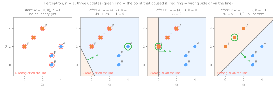
Perceptron on six points: after A the line is 4x1 + 2x2 + 1 = 0, after B it is x1 = 0, after C it is x2 = x1 − 1/3, which separates the classes

\(w\) is perpendicular to the line and points to the \(+1\) side. A mistake on a \(-1\) point subtracts it from \(w\); on a \(+1\) point, adds it. If a margin \(\gamma\) exists, at most \((R/\gamma)^2\) mistakes (Novikoff, 1962), but at some line, not the best one.

Simulator: the perceptron

Step visits one point and shows the arithmetic. Predict. On the third preset (XOR), will the mistakes per epoch ever reach zero?

Stage 2 · why is one line not enough, and what do layers add?

XOR: why one line is not enough

\((0, 1)\) and \((1, 0)\) are \(+1\); \((0, 0)\) and \((1, 1)\) are \(-1\). A separating line would need:

\((0,0)\) negative: \(b < 0\)
\((0,1)\), \((1,0)\) positive: \(w_2 + b > 0\), \(w_1 + b > 0\)
\((1,1)\) negative: \(w_1 + w_2 + b < 0\)

Add the middle two: \(w_1 + w_2 + 2b > 0\), so \(w_1 + w_2 + b > -b > 0\). Contradiction.

The perceptron makes 4 mistakes per epoch, for ever: the four updates of an epoch add up to exactly zero. Minsky and Papert, Perceptrons (1969).

The same wall stops logistic regression

A noisy XOR: 400 points around the four corners (205 and 195 per class), 5-fold cross-validation.

logistic regression

0.485

CV accuracy: chance level

its probabilities

0.37–0.61

P(class 1) everywhere: it hedges

Predict. XOR is "\(x_1\) OR \(x_2\), but NOT both". Each piece is linearly separable. How could several neurons solve it?

A hidden layer solves XOR

\(h_1\): \(x_1 + x_2 - 0.5 > 0\), OR
\(h_2\): \(x_1 + x_2 - 1.5 > 0\), AND
output: \(h_1 - h_2 - 0.5 > 0\), XOR

\(x_1\)	\(x_2\)	\(h_1\)	\(h_2\)	\(z_{\text{out}}\)	out
0	0	0	0	−0.5	0
0	1	1	0	0.5	1
1	0	1	0	0.5	1
1	1	1	1	−0.5	0

Row \((1, 1)\): \(z_1 = 1.5 \Rightarrow h_1 = 1\); \(z_2 = 0.5 \Rightarrow h_2 = 1\); \(z_{\text{out}} = 1 - 1 - 0.5 = -0.5 \Rightarrow 0\). Every weight chosen by hand.

The hidden layer builds new features

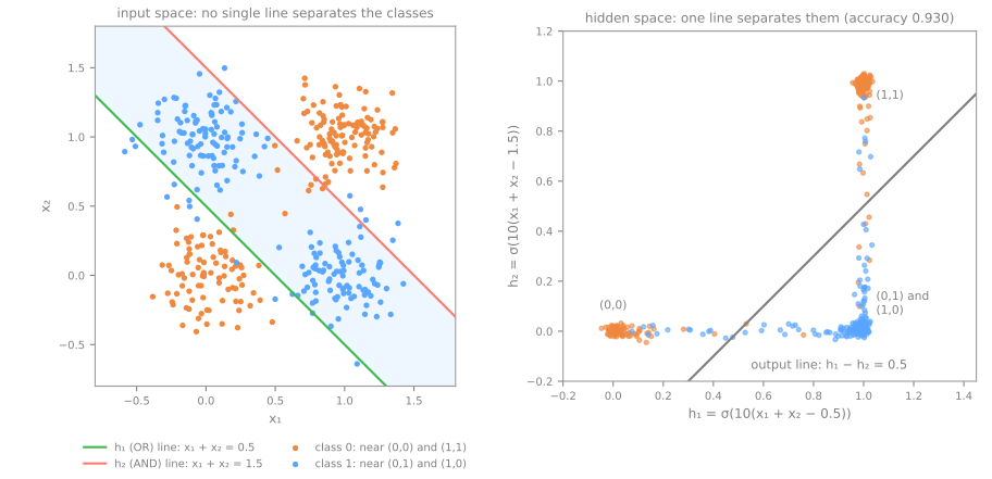
Left: the noisy XOR with the OR and AND lines; class 1 lies between them. Right: in the hidden space the points fall on three corners and one line separates the classes

The hidden layer computes features in which the problem becomes linearly separable; the output is a linear classifier on them. Polynomial features did it by hand, the SVM kernel implicitly: a network learns them.

From step to sigmoid: something to differentiate

The step has derivative 0 everywhere: the gradient says nothing. Replace it by a sigmoid and multiply every weight by 10:

\(x_1\)	\(x_2\)	\(h_1\)	\(h_2\)	P(XOR = 1)
0	0	0.007	0.000	0.007
0	1	0.993	0.007	0.992
1	0	0.993	0.007	0.992
1	1	1.000	0.993	0.007

The same network, now differentiable: the kind a gradient-based trainer can find by itself.

Activation functions

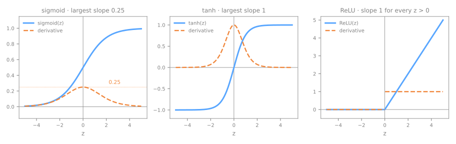
Sigmoid, tanh and ReLU with their derivatives: the sigmoid's slope never exceeds 0.25; tanh peaks at 1; ReLU has slope 1 for every positive input

	largest derivative
sigmoid	0.25, at \(z = 0\)
tanh	1, at \(z = 0\)
ReLU	1, for every \(z > 0\)

Backpropagation multiplies one derivative per layer: through 10 sigmoid layers at most \(0.25^{10} \approx 10^{-6}\). The vanishing gradient is why ReLU is the default for hidden layers.

Without a nonlinearity, layers collapse

\(W_2 (W_1 x + b_1) + b_2\) is one layer with weights \(W_2 W_1\): a linear function of a linear function is linear.

two linear layers

−5.4084

one merged layer

−5.4084

ReLU between

−5.3273

On the noisy XOR, 8 hidden units:

activation	CV accuracy
`identity`	0.510
`relu`	0.983

Stage 3 · what does a network compute?

The forward pass: one matrix product per layer

\[ z = W x + b^{h}, \quad h = \sigma(z), \quad u = v^\top h + b^{y}, \quad \hat{y} = \sigma(u) \]

For a batch: \(H = \sigma(X W^\top + b^h)\). That is why networks run so well on GPUs, machines for multiplying matrices.

a 2-2-1 network, one example \(x = (0.5, 0.8)\), target \(y = 0\)

\(W = \begin{pmatrix} 0.2 & 0.4 \\ 0.6 & 0.8 \end{pmatrix}\), \(b^h = (0.1, 0.2)\), \(v = (0.3, 0.5)\), \(b^y = 0.4\)

Predict. The target is 0. Will the network's output be close to 0?

The 2-2-1 network, by hand

\(z_1 = 0.2 \cdot 0.5 + 0.4 \cdot 0.8 + 0.1 = 0.52\)

\(z_2 = 0.6 \cdot 0.5 + 0.8 \cdot 0.8 + 0.2 = 1.14\)

\(h = \sigma(z) = (0.627, 0.758)\)

\(u = 0.3 \cdot 0.627 + 0.5 \cdot 0.758 + 0.4 = 0.967\)

\(\hat y = \sigma(0.967) = 0.725\)

squared loss

0.5249

\(L = (0.725 - 0)^2\): quite wrong

scikit-learn, with the same weights loaded: 0.7245

Counting parameters

A layer: \((n_\text{in} + 1) \cdot n_\text{out}\) parameters.

architecture	parameters
2 → 2 → 1	9
64 → 10	650
64 → 32 → 10	2,410
64 → 256 → 10	19,210
64 → 64 → 64 → 10	8,970

256 units: more parameters than images in the whole digits dataset (1,797). The count grows with the product of neighboring widths; regularization is not optional.

Stage 4 · how does it learn every weight at once?

Backpropagation: the chain rule, organized

\[ w_{11} \;\to\; z_1 \;\to\; h_1 \;\to\; u \;\to\; \hat y \;\to\; L \]

loss gradient: \(\partial L / \partial \hat y = 2(\hat y - y)\)
output delta: \(\delta_y = 2(\hat y - y) \cdot \hat y (1 - \hat y)\)
output weights: \(\partial L / \partial v_{1j} = \delta_y \, h_j\)
hidden deltas: \(\delta_{h_j} = \delta_y \, v_{1j} \cdot h_j (1 - h_j)\)
hidden weights: \(\partial L / \partial w_{jk} = \delta_{h_j} \, x_k\)
update: \(p \leftarrow p - \eta \, \partial L / \partial p\)

Every weight's gradient = the delta of the unit it feeds × the value that came into it. Rumelhart, Hinton & Williams (1986).

The six steps, with numbers

step	value	reading
1. \(\partial L/\partial \hat y\)	1.449	push \(\hat y\) down toward 0
2. \(\delta_y\)	0.2892	\(1.449 \times 0.199\), the output sigmoid's slope
3. \(\partial L/\partial v\)	0.1814, 0.2191	larger for \(h_2 = 0.758\), which contributed more
4. \(\delta_h\)	0.0203, 0.0266	ten times smaller: weights < 1 and slopes < 0.25
5. \(\partial L/\partial W\)	0.0101 to 0.0212	the smallest: the vanishing gradient, in miniature

Finite differences agree to \(1.3 \times 10^{-10}\): backpropagation is the exact derivative. One step with \(\eta = 0.5\): loss 0.5249 → 0.4405.

Simulator: backpropagation, step by step

Step 1 is the forward pass; steps 2 to 6 send the gradient back; step 7 updates with \(\eta = 0.5\). Use Next and Back (click the simulator to use the arrow keys inside it).

Why backpropagation matters: the cost

finite differences

2 extra forward passes per parameter: 18 for the 9 parameters; 4,820 for a 64-32-10 digit network

backpropagation

one backward pass for all the gradients, about the cost of the forward pass

With cross-entropy, steps 1 and 2 collapse into \(\delta_y = \hat y - y\): the same "prediction minus target" as logistic regression.

Non-convex: the starting point matters

The noisy XOR, 10 random starts (random_state 0–9), training accuracy:

hidden units	seeds 0–9
2	0.76 0.66 0.74 0.94 0.94 0.94 0.94 0.94 0.74 0.66
8	0.98 0.98 0.97 0.98 0.98 0.96 0.99 0.99 0.97 0.95

With 2 units, half the starts get stuck in a worse local minimum. Extra units give gradient descent more routes, one reason networks are wider than the minimum. Check conclusions over a few seeds.

Optimizers and regularization

`adam`

the default: mini-batches of 200 with momentum and a per-parameter step

`sgd`

plain mini-batch gradient descent, optional momentum

`lbfgs`

whole training set, curvature; best on small datasets

alpha: weight decay, the L2 penalty of Ridge on every weight.
early_stopping=True: hold out 10%, stop after 10 epochs without improvement.
dropout in deep-learning libraries; not in scikit-learn.

Stage 5 · how do we train it well, and when is it worth it?

In practice: scale the inputs

Spambase: 4,601 e-mails, 57 features, standard deviations from 0.076 to 606.

MLP	CV accuracy
raw inputs	0.927
`StandardScaler` first	0.948

Two points from one line of preprocessing, inside the pipeline. Unscaled features stretch the loss surface into a narrow valley, as for linear models.

Width and weight decay, on noisy moons

Predict. 1, 3, 10 or 100 hidden units, almost no penalty: which has the best cross-validation accuracy?

hidden units	train	CV
logistic regression		0.830
1	0.842	0.843
3	0.897	0.873
10	0.938	0.893
100	0.997	0.857

100 units, `alpha`	train	CV
0.0001	0.997	0.857
0.01	0.993	0.880
0.1	0.939	0.903
1	0.914	0.917
10	0.837	0.830

The boundaries

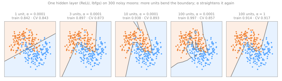
Decision boundaries on noisy moons: 1 unit draws a line, 3 and 10 units bend it, 100 units wrap single points, 100 units with alpha = 1 give a smooth curve

The recipe of every model in this course: a generous architecture, then tune alpha (and the width) with cross-validation.

Depth, and when to use a network

One hidden layer is a universal approximator (Cybenko, 1989; Hornik, 1991): existence, not that training finds it.
Deep networks build on previous layers: edges → textures → objects. That hierarchy took over perception from 2012 on.

spambase, same folds	mean	std
logistic	0.924	0.008
MLP	0.948	0.005
MLP early stop	0.942	0.006
gradient boosting	0.956	0.011

On tables, tree ensembles stay as good or better, with defaults and no preprocessing. On images, audio and text, the balance flips.

Summary

A neuron = weighted sum + activation; with a sigmoid, logistic regression.
One neuron draws one line: XOR needs a hidden layer, which learns new features.
Nonlinear activations, or layers collapse; ReLU fights the vanishing gradient.
Backpropagation: deltas sent backwards, the exact gradient in one pass.
Non-convex: seeds matter. Scale, then tune width and alpha by cross-validation.

Next: the Deep Learning course continues from exactly here.

Lab

A neural network on handwritten digits

1,797 digits, 8 × 8 pixels: name the digit. Download the lab notebook and open it in Jupyter or Colab; it runs in about a minute.
Lock the test set away; compare a baseline and three models on the same folds.
Tune the width and alpha; read the loss curve and early stopping.
Is the MLP really better, fold by fold? Then touch the test set once.