Pipelines
The preprocessing lesson set a rule: every step that learns something from the data (the median of an imputer, the mean and standard deviation of a scaler, the list of categories of an encoder) is fit on the training rows only, and then replayed, unchanged, on every other row the model will ever see: the test set, a validation split, next month's data in production. Written by hand, that rule becomes a pile of fit and transform calls that must stay in the right order, on the right data, forever. This lesson measures what goes wrong when one of those calls slips, and replaces the pile with a single object, scikit-learn's Pipeline, that makes the rule impossible to break by accident.
The lesson tells that story in four stages, drawn below: 1. the manual workflow, seven calls and three bugs, each one measured; 2. one Pipeline, which removes the three bugs by construction; 3. real columns, with ColumnTransformer routing each group of columns to its own treatment and steps of your own; 4. inspect and trust, opening and saving the fitted object and measuring the leak it prevents. Each stage links to its section, and in the slides a strip at the bottom shows which stage you are in.
- The manual workflowseven calls, three bugs, measured
- One Pipelinefit and predict, step by step
- Real columnsColumnTransformer and steps of your own
- Inspect and trustinspection, persistence, the leak it prevents
Every number below comes from running the code on this page; each figure is produced by a short script that sits next to it.
Slides
Click the slides and use the ← → arrows to navigate; F goes full screen and Esc shows every slide. Open the slides in a new tab
The problem pipelines solve
The manual workflow
Stage 1. The data is the California housing table from the EDA lesson: 20,640 districts, eight numeric columns (one of them, total_bedrooms, with missing values), one categorical column (ocean_proximity) and the target, the median house value of the district. To keep the start simple, the first sections use only the eight numbers. The preprocessing is the one from the previous lesson: fill the holes with the median, then standardize.
import numpy as np
import pandas as pd
from sklearn.impute import SimpleImputer
from sklearn.metrics import mean_absolute_error
from sklearn.model_selection import train_test_split
from sklearn.neighbors import KNeighborsRegressor
from sklearn.preprocessing import StandardScaler

url = "https://raw.githubusercontent.com/hsandmann/biblio/refs/heads/main/ml/aula02/housing.csv"
housing = pd.read_csv(url)
X = housing.drop(columns='median_house_value')          # 9 columns: 8 numbers + ocean_proximity
y = housing['median_house_value']
X_train, X_test, y_train, y_test = train_test_split(X, y, test_size=0.2, random_state=42)
num = ['longitude', 'latitude', 'housing_median_age', 'total_rooms',
       'total_bedrooms', 'population', 'households', 'median_income']

# the manual workflow: three objects, each fit on train, then replayed on test
imputer = SimpleImputer(strategy='median')
scaler = StandardScaler()
model = KNeighborsRegressor(n_neighbors=10)              # black box: see the note below

A_train = scaler.fit_transform(imputer.fit_transform(X_train[num]))   # learn on train
model.fit(A_train, y_train)
A_test = scaler.transform(imputer.transform(X_test[num]))             # replay on test
pred = model.predict(A_test)

def mae(p):
    return f"${mean_absolute_error(y_test, p):,.0f}"

print(f"{len(X_train)} training districts, {len(X_test)} test districts")
print("MAE, careful manual workflow:", mae(pred))
print("MAE, always the training mean:", mae(np.full(len(y_test), y_train.mean())))
16512 training districts, 4128 test districts
MAE, careful manual workflow: $43,023
MAE, always the training mean: $92,894
The model is a black box in this lesson
KNeighborsRegressor predicts the value of a district as the average of the 10 most similar training districts, where "similar" means close in the eight standardized numbers. You will study it properly in the k-NN lesson; here it only needs two properties. It depends on the scale of the columns, so preprocessing mistakes show up in its predictions. And it is fast. Any other model would do for the pipeline mechanics.
The score is the mean absolute error (MAE): on average, the prediction misses the true value of a test district by $43,023. A "model" that ignores the district and always answers the training mean misses by $92,894. That is the floor any real model must beat.
The careful version takes seven calls on three objects, and the order matters in both directions: fit_transform on train, transform on test, imputer before scaler, the same eight columns in the same order. Each of the three classic bugs below changes one thing in the prediction code. The trained model is the same in every case.
Bug 1 — re-fitting on the data you predict
The most common slip is one word: fit_transform where transform was meant. The step then re-learns its statistics from the rows it is supposed to transform. It is easiest to see by hand. Take one column with five training rows and two new rows:
| training rows | new rows |
|---|---|
| 200, NaN, 400, 600, 800 | NaN, 900 |
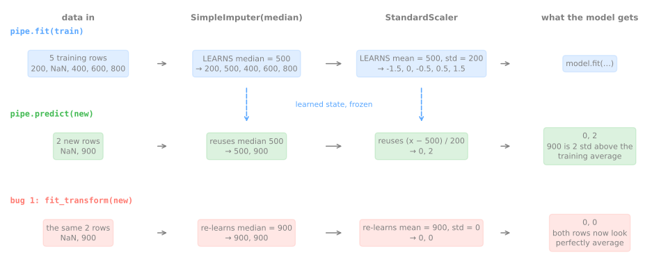
Fit on the training rows. The median of the four known values is \((400 + 600)/2 = 500\), so the imputed column is 200, 500, 400, 600, 800. Its mean is 500 and its standard deviation is \(\sqrt{(300^2 + 0^2 + 100^2 + 100^2 + 300^2)/5} = \sqrt{40{,}000} = 200\). The new rows become: NaN → 500 → \((500 - 500)/200 = 0\), and 900 → \((900 - 500)/200 = 2\). The second new district is two standard deviations above the training average, which is information the model can use.
Re-fit on the new rows instead. Their median is 900 (the only known value), so both rows become 900; their mean is 900 and their spread is zero; both are transformed to 0. The district with 900 bedrooms, two standard deviations above the training average, now looks perfectly average. scikit-learn agrees:
toy_train = pd.DataFrame({'total_bedrooms': [200, np.nan, 400, 600, 800]})
toy_new = pd.DataFrame({'total_bedrooms': [np.nan, 900]})

imp, sc = SimpleImputer(strategy='median'), StandardScaler()
sc.fit(imp.fit_transform(toy_train))                       # learn on the 5 training rows
print("learned: median", imp.statistics_, "mean", sc.mean_, "std", sc.scale_)
print("right: transform         ", sc.transform(imp.transform(toy_new)).ravel())
print("wrong: fit_transform again", StandardScaler().fit_transform(
                                    SimpleImputer(strategy='median').fit_transform(toy_new)).ravel())
learned: median [500.] mean [500.] std [200.]
right: transform          [0. 2.]
wrong: fit_transform again [0. 0.]
(When a column has no spread at all, StandardScaler divides by 1 instead of 0, so the result is 0 rather than an error.)
How much this costs on the real data depends on how the rows arrive for prediction. In a notebook, the whole test set arrives at once. In production, rows arrive in batches (one region's office sends its districts) or one at a time (a user fills in a form). The function below reproduces the bug: the trained model is the same, but the scaler is re-fit on each batch it predicts.
def predict_bug1(batch):
    """BUG 1: fit_transform where transform was meant: the scaler re-learns on the batch."""
    return model.predict(StandardScaler().fit_transform(imputer.transform(batch[num])))

print("re-fit on the whole test set:  ", mae(predict_bug1(X_test)))
by_region = pd.concat([pd.Series(predict_bug1(batch), index=batch.index)
                       for _, batch in X_test.groupby('ocean_proximity')])
print("re-fit on each region's batch: ", mae(by_region[X_test.index]))
one_by_one = [predict_bug1(X_test.iloc[[i]])[0] for i in range(len(X_test))]
print("re-fit on one district at a time:", mae(one_by_one),
      f"({len(set(one_by_one))} distinct prediction)")
re-fit on the whole test set:   $42,814
re-fit on each region's batch:  $65,754
re-fit on one district at a time: $116,049 (1 distinct prediction)
Three results, one bug:
- On the whole test set the bug is invisible. 4,128 random districts have almost the same means and standard deviations as the 16,512 training districts, so re-fitting changes almost nothing, and the MAE even comes out $209 lower than the correct one, by chance. This is why the bug survives code review: the notebook looks fine.
- On regional batches it costs $22,731 per district. Each batch is re-centered on itself. Inland districts are measured against other inland districts, so an income that is modest by the standards of the state becomes "average", and the latitude and longitude of every batch are moved to the center of the map. The neighbors the model finds are no longer the right ones.
- One district at a time, the model is worse than useless. A single row has zero spread, so every column becomes 0 (the toy table above). Every district is the same point, gets the same 10 neighbors and the same prediction: one distinct value for 4,128 districts, and an MAE of $116,049, worse than always predicting the mean.
Bug 2 — a step forgotten at prediction time
Training code and prediction code are often written at different times, by different people, sometimes in different files. A step present in one and missing in the other is the second classic:
print("scaler forgotten:", mae(model.predict(imputer.transform(X_test[num]))))
try:
    model.predict(scaler.transform(X_test[num]))           # imputer forgotten
except ValueError as err:
    print("imputer forgotten:", str(err).splitlines()[0])
Forgetting the imputer is the lucky case: the missing values reach the model and it refuses them with an error. Forgetting the scaler is silent. The model receives raw numbers (a total_rooms of 2,000 where it learned values of a few units around 0), computes distances dominated by the largest columns, and returns a confident prediction for every district. The MAE, $105,978, is again worse than predicting the mean, and nothing on the screen says so.
Bug 3 — a different column order
The model receives numbers, not names: column 5 of the array is "population" only because it was column 5 during training. If the data arrives in another order (a new export from the database, a different API client), each column gets the statistics and the neighbors of another. Here two count columns trade places:
swapped = ['longitude', 'latitude', 'housing_median_age', 'total_rooms',
           'total_bedrooms', 'households', 'population', 'median_income']   # last-but-two swapped
X_new = X_test[swapped]
print("swapped, sent as an array:", mae(model.predict(scaler.transform(imputer.transform(X_new.to_numpy())))))
try:
    imputer.transform(X_new)                                # sent as a DataFrame
except ValueError as err:
    print("swapped, sent as a DataFrame:", " ".join(str(err).splitlines()[:2]))
swapped, sent as an array: $101,517
swapped, sent as a DataFrame: The feature names should match those that were passed during fit. Feature names must be in the same order as they were in fit.
As an array, the swap costs $101,517 per district. A district has about three times more residents than households, so the "households" column is suddenly three times larger than anything the model saw and the "population" column three times smaller. The only hint is a UserWarning ("X does not have valid feature names") among the usual notebook warnings. As a DataFrame, scikit-learn compares the column names with the ones it saw in fit and refuses. Keep the data in a DataFrame all the way to the model, and let the first step check the names.
The figure puts the six results side by side (figure script):
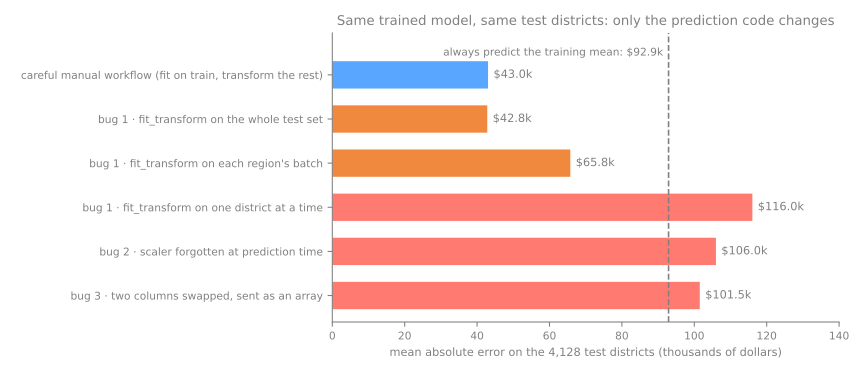
Three of the six bars are worse than the baseline that ignores the data, and the most dangerous bar is the second one, the bug that looks correct.
Pipeline: one estimator, many steps
Stage 2. A Pipeline is a list of steps that behaves as a single estimator. make_pipeline builds one from the steps and names them automatically:
from sklearn.pipeline import make_pipeline

pipe = make_pipeline(SimpleImputer(strategy='median'), StandardScaler(),
                     KNeighborsRegressor(n_neighbors=10))
pipe.fit(X_train[num], y_train)            # every step learns from the training rows
pred_pipe = pipe.predict(X_test[num])      # every step replays what it learned
print("MAE:", mae(pred_pipe), "· identical to the careful manual workflow:",
      np.array_equal(pred_pipe, pred))

one_by_one = [pipe.predict(X_test[num].iloc[[i]])[0] for i in range(len(X_test))]
print("one district at a time == all at once:", np.allclose(one_by_one, pred_pipe))
try:
    pipe.predict(X_new)                    # the swapped columns of bug 3
except ValueError as err:
    print("swapped columns:", str(err).splitlines()[0])
print(list(pipe.named_steps))
MAE: $43,023 · identical to the careful manual workflow: True
one district at a time == all at once: True
swapped columns: The feature names should match those that were passed during fit.
['simpleimputer', 'standardscaler', 'kneighborsregressor']
Two calls, fit and predict, replace seven, the predictions are exactly those of the careful manual workflow, and the three bugs are gone by construction:
- Bug 1.
pipe.predictnever callsfiton a transformer, so the batch size stops mattering: 4,128 predictions made one district at a time are identical to the 4,128 made at once. - Bug 2. There is no separate prediction code in which to forget a step. The steps travel inside the object.
- Bug 3. The pipeline hands the DataFrame to its first step, which checks the column names and refuses the swapped table.
The rules of composition are few. Every step except the last must be a transformer (it has fit and transform); the last step can be anything with fit, usually a model with predict. The pipeline then exposes the methods of its last step: pipe.predict, pipe.score, and pipe.predict_proba for a classifier.
What fit and predict do, step by step
pipe.fit(X, y) walks down the list. Each transformer is fit on what it receives and then transforms it (fit_transform); its output is the input of the next step; the last step is only fit. pipe.predict(X) walks the same list calling only transform, with the parameters frozen at fit time, and ends with the model's predict. The toy column of bug 1, drawn as a pipeline (figure script):
To watch it happen on the real data, put a do-nothing step that reports what it sees between the real steps (how to write such a class is the subject of your own steps, below). It prints the shape of the data and, for the total_bedrooms column, the number of missing values and the mean at that point:
from sklearn.base import BaseEstimator, TransformerMixin

class Spy(BaseEstimator, TransformerMixin):
    """A step that changes nothing and reports what passes through it."""
    def __init__(self, label=''):
        self.label = label

    def fit(self, X, y=None):
        self._report('fit', X)
        return self

    def transform(self, X):
        self._report('transform', X)
        return X

    def _report(self, call, X):
        X = np.asarray(X, dtype=float)
        col = X[:, 4]                                            # total_bedrooms
        print(f"  {self.label:8s} {call:9s} {str(X.shape):11s} "
              f"missing {np.isnan(col).sum():3d} · mean {np.nanmean(col):7.2f}")

traced = make_pipeline(Spy('raw'), SimpleImputer(strategy='median'), Spy('imputed'),
                       StandardScaler(), Spy('scaled'), KNeighborsRegressor(n_neighbors=10))
print("traced.fit(X_train, y_train)")
traced.fit(X_train[num], y_train)
print("traced.predict(X_test)")
_ = traced.predict(X_test[num])
traced.fit(X_train, y_train)
  raw      fit       (16512, 8)  missing 163 · mean  538.92
  raw      transform (16512, 8)  missing 163 · mean  538.92
  imputed  fit       (16512, 8)  missing   0 · mean  537.92
  imputed  transform (16512, 8)  missing   0 · mean  537.92
  scaled   fit       (16512, 8)  missing   0 · mean    0.00
  scaled   transform (16512, 8)  missing   0 · mean    0.00
traced.predict(X_test)
  raw      transform (4128, 8)   missing  44 · mean  533.66
  imputed  transform (4128, 8)   missing   0 · mean  532.63
  scaled   transform (4128, 8)   missing   0 · mean   -0.01
Read it from top to bottom:
- During
fit, only training rows exist. Every step sees 16,512 rows, never 4,128. Each step is fit and then immediately transforms (thefit+transformpairs), because the next step must be fit on transformed training data: the scaler learns its mean from imputed values (537.92), not from raw ones with holes. - The imputer fills 163 holes with the training median, which pulls the mean of the column down by one bedroom, from 538.92 to 537.92: the median (437) is below the mean because the column has a long right tail.
- During
predict, nobody callsfit. The 44 holes of the test set are filled with the training median, and the scaler subtracts the training mean. That is why the scaled test column has mean −0.01 and not exactly 0: the test rows are measured with the ruler of the training rows, which is the honest thing to do. A mean of exactly 0.00 on the test set would be the symptom of bug 1.
Pipeline or make_pipeline
make_pipeline names each step after its class, in lower case: 'simpleimputer', 'standardscaler', 'kneighborsregressor' (and 'spy-1', 'spy-2', ... when a class repeats). Pipeline takes the names from you, as a list of (name, step) pairs:
from sklearn.pipeline import Pipeline

pipe_named = Pipeline([('impute', SimpleImputer(strategy='median')),
                       ('scale', StandardScaler()),
                       ('model', KNeighborsRegressor(n_neighbors=10))])
Both build the same kind of object; the names only matter when you refer to a step later (to inspect it, or to change one of its settings). Short explicit names pay off in long pipelines.
Heterogeneous columns: ColumnTransformer
Stage 3. A pipeline applies every step to every column. Real tables need different treatments for different columns: here the eight numbers need the median and the scaler, and ocean_proximity, a text column, needs one-hot encoding. A ColumnTransformer routes each group of columns to its own branch and puts the results side by side:
from sklearn.compose import ColumnTransformer
from sklearn.preprocessing import OneHotEncoder

preprocess = ColumnTransformer([
    ('num', make_pipeline(SimpleImputer(strategy='median'), StandardScaler()), num),
    ('cat', OneHotEncoder(handle_unknown='ignore', sparse_output=False), ['ocean_proximity']),
])
full = make_pipeline(preprocess, KNeighborsRegressor(n_neighbors=10))
full.fit(X_train, y_train)                 # the raw 9-column table goes in
print("MAE with ocean_proximity:", mae(full.predict(X_test)))
print(preprocess.get_feature_names_out())
MAE with ocean_proximity: $41,552
['num__longitude' 'num__latitude' 'num__housing_median_age'
 'num__total_rooms' 'num__total_bedrooms' 'num__population'
 'num__households' 'num__median_income' 'cat__ocean_proximity_<1H OCEAN'
 'cat__ocean_proximity_INLAND' 'cat__ocean_proximity_ISLAND'
 'cat__ocean_proximity_NEAR BAY' 'cat__ocean_proximity_NEAR OCEAN']
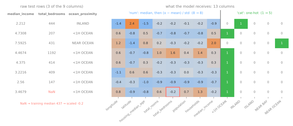
Each branch is a triple (name, transformer, columns), and a branch can itself be a pipeline, as 'num' is. The whole thing is one transformer, so it goes into a pipeline like any other step, and the model now receives the raw 9-column table: the text column is no longer a problem, and using it lowers the MAE from $43,023 to $41,552.
get_feature_names_out says what each output column is. The prefix is the name of the branch that produced it (num__, cat__), and the one-hot columns carry the category (cat__ocean_proximity_INLAND). Without it, the model's input is a 13-column block of anonymous numbers. What actually comes out, for eight test districts (figure script):
Which columns go where: lists, remainder, selectors
Columns that no branch mentions are dropped by default (remainder='drop'). With remainder='passthrough' they are appended unchanged:
two = ColumnTransformer([('num', StandardScaler(), ['median_income', 'housing_median_age'])])
print("remainder='drop':       ", two.fit_transform(X_train).shape)
two_plus = ColumnTransformer([('num', StandardScaler(), ['median_income', 'housing_median_age'])],
                             remainder='passthrough')
print("remainder='passthrough':", two_plus.fit_transform(X_train).shape)
print(two_plus.get_feature_names_out()[:4])
remainder='drop':        (16512, 2)
remainder='passthrough': (16512, 9)
['num__median_income' 'num__housing_median_age' 'remainder__longitude'
 'remainder__latitude']
'drop' is the safe default: an identifier column or a free-text field you forgot about never reaches the model silently. 'passthrough' is for columns that are already ready. Here it would be a mistake, because the seven passed-through columns arrive unscaled (and ocean_proximity arrives as text).
Instead of lists of names, a branch can take a selector that chooses columns by type when the transformer is fit:
from sklearn.compose import make_column_selector

by_type = ColumnTransformer([
    ('num', make_pipeline(SimpleImputer(strategy='median'), StandardScaler()),
     make_column_selector(dtype_include='number')),
    ('cat', OneHotEncoder(handle_unknown='ignore', sparse_output=False),
     make_column_selector(dtype_exclude='number')),
])
by_type.fit(X_train)
for name, _, columns in by_type.transformers_:
    print(name, columns)
num ['longitude', 'latitude', 'housing_median_age', 'total_rooms', 'total_bedrooms', 'population', 'households', 'median_income']
cat ['ocean_proximity']
The fitted transformer (transformers_, with the trailing underscore) records the columns each selector picked. Selectors are convenient for wide tables, but they trust the types: a zip code stored as a number lands in the numeric branch. Explicit lists are more work and say exactly what happens.
Seeing the output: feature names and set_output
By default a transformer returns a NumPy array. set_output(transform='pandas') makes it return a DataFrame with the names of get_feature_names_out as columns, which is the easiest way to check a preprocessing by eye:
                                 20046  3024   15663
num__longitude                   -1.41   0.60   1.16
num__latitude                     2.36  -0.84  -1.36
num__housing_median_age          -1.47   0.51   0.82
num__total_rooms                 -0.17  -0.67   0.21
num__total_bedrooms              -0.23  -0.80  -0.26
num__population                  -0.14  -0.73  -0.22
num__households                  -0.16  -0.76  -0.18
num__median_income               -0.87   0.45   1.96
cat__ocean_proximity_<1H OCEAN    0.00   1.00   0.00
cat__ocean_proximity_INLAND       1.00   0.00   0.00
cat__ocean_proximity_ISLAND       0.00   0.00   0.00
cat__ocean_proximity_NEAR BAY     0.00   0.00   0.00
cat__ocean_proximity_NEAR OCEAN   0.00   0.00   1.00
Three test districts, transposed so that each column of the output is a row here. District 20046 is inland, 2.36 standard deviations north of the average training district, with an income 0.87 standard deviations below average. The index of the DataFrame is preserved, so every transformed row can be traced back to its raw row. (pandas output needs dense arrays, hence sparse_output=False in the encoder.)
Robust to column order and to new categories
A ColumnTransformer fit on a DataFrame selects its columns by name, so bug 3 goes away completely instead of turning into an error. And an encoder with handle_unknown='ignore' turns a category it never saw into a row of zeros instead of crashing:
reversed_cols = X_test[X_test.columns[::-1]]              # same columns, opposite order
print("reversed columns, same predictions:", np.array_equal(full.predict(reversed_cols), full.predict(X_test)))
new = X_test.head(1).assign(ocean_proximity='LAKE')        # a category never seen in training
print(preprocess.transform(new).filter(like='ocean').to_numpy(), full.predict(new).round())
With all nine columns in reverse order, the predictions are identical. The district relabeled 'LAKE' gets zeros in the five ocean_proximity columns and a prediction, $90,030, the same as with its real label, INLAND: its 10 nearest neighbors are so close in the eight numbers that losing one category column did not change them. Without handle_unknown='ignore', the same row would raise ValueError: Found unknown categories, and one new value in production would take the whole service down. Rare categories make this likely even without typos: ISLAND has 5 districts in the whole table, all of which landed in the training set with this split.
Your own steps
Anything that learns from data and transforms it can become a pipeline step. There are two ways, depending on whether the step has something to learn.
Stateless: FunctionTransformer
The preprocessing lesson recommended \(\log(1 + x)\) for right-skewed columns. A logarithm learns nothing from the data, so FunctionTransformer turns the function into a step directly:
from sklearn.preprocessing import FunctionTransformer

counts = ['total_rooms', 'total_bedrooms', 'population', 'households']
log = FunctionTransformer(np.log1p, feature_names_out='one-to-one')   # nothing to learn
print("skewness before:", X_train[counts].skew().round(2).to_list())
print("skewness after: ", log.fit_transform(X_train[counts]).skew().round(2).to_list())
The four count columns go from a strong right skew (3.3 to 5.2) to a milder left skew (about −1). Its fit does nothing, so it cannot leak. feature_names_out='one-to-one' tells the step that output column i is input column i, so get_feature_names_out keeps working after it.
Stateful: a transformer of your own
When the step must learn something, it needs a class with fit and transform. The example is a clipper. total_rooms goes up to 39,320 in a table whose median is about 2,100, and a single extreme value, or a typo in new data, can dominate the distances of the model. The clipper learns, on the training rows only, the 1st and 99th percentiles of each column, and pulls every value outside that range back to the nearest bound:
from sklearn.base import OneToOneFeatureMixin
from sklearn.utils.validation import check_is_fitted, validate_data

class Clipper(OneToOneFeatureMixin, TransformerMixin, BaseEstimator):
    """Clip each column to percentiles learned on the training data."""
    def __init__(self, low=1, high=99):
        self.low = low                     # hyperparameters: stored as given, nothing else
        self.high = high

    def fit(self, X, y=None):
        X = validate_data(self, X)         # to an array; remembers the column names and count
        self.lower_ = np.percentile(X, self.low, axis=0)     # learned state ends with "_"
        self.upper_ = np.percentile(X, self.high, axis=0)
        return self

    def transform(self, X):
        check_is_fitted(self)
        X = validate_data(self, X, reset=False)             # same columns as in fit, or an error
        return np.clip(X, self.lower_, self.upper_)

clipped = make_pipeline(
    ColumnTransformer([
        ('num', make_pipeline(SimpleImputer(strategy='median'), Clipper(), StandardScaler()), num),
        ('cat', OneHotEncoder(handle_unknown='ignore', sparse_output=False), ['ocean_proximity'])]),
    KNeighborsRegressor(n_neighbors=10))
clipped.fit(X_train, y_train)
clip = clipped[0].named_transformers_['num'][1]
print(pd.DataFrame({'lower_': clip.lower_, 'upper_': clip.upper_}, index=num).round(1))
print("MAE:", mae(clipped.predict(X_test)))
                    lower_   upper_
longitude           -123.2   -116.3
latitude              32.7     40.6
housing_median_age     4.0     52.0
total_rooms          162.2  11248.0
total_bedrooms        35.0   2245.6
population            88.0   5825.3
households            30.0   2006.6
median_income          1.1     10.7
MAE: $41,361
The conventions are what make a class a scikit-learn step:
__init__only stores the hyperparameters, under the same names as the arguments, and does nothing else.BaseEstimatorreads them from there to provideget_params,set_paramsand the printed representation.fitlearns and returnsself. Everything learned from data gets a name that ends with an underscore (lower_,upper_), the same convention asmean_andstatistics_.validate_dataconverts the input to an array and records the number and names of the columns.transformapplies what was learned, after checking that the object was fit and that the columns are the same.TransformerMixinprovidesfit_transform(andset_output);OneToOneFeatureMixinprovidesget_feature_names_outfor a step that keeps its columns one to one.
The table is the learned state: the bounds come from the 16,512 training districts. On this test set, the clipper improves the MAE only slightly, from $41,552 to $41,361, because few test values are outside the bounds. Its real job is protection against values nobody has seen. Take the first test district and multiply its total_rooms by 1,000, a unit error of the kind that appears when a new data source starts sending rooms in a different unit:
typo = X_test.head(1).copy()
typo['total_rooms'] *= 1000                # a unit error in one new row
print(f"true value ${y_test.iloc[0]:,.0f} · correct row ${full.predict(X_test.head(1))[0]:,.0f}")
print(f"with the typo: no clipper ${full.predict(typo)[0]:,.0f} · clipper ${clipped.predict(typo)[0]:,.0f}")
Sweeping the multiplier from 1 to 1,000 shows where the difference comes from (figure script):
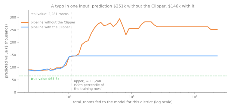
Up to 11,248 rooms (the learned upper_) the two pipelines almost agree. Beyond it, the unclipped pipeline follows the typo into regions of the data where the only neighbors are huge districts, and its prediction wanders up to $251,020. The clipped one sees at most 11,248 and stays at $145,690. That is still a wrong answer for a district worth $65,600, and no transformer can fix bad input. But the damage is bounded, and the bound was learned from training data only.
Inspection and persistence
Stage 4. A fitted pipeline is a container you can open. Steps are reached by name (named_steps) or by position, with the same indexing as a Python list, and a slice is a smaller pipeline:
print(list(full.named_steps))
print(full[-1])                                           # indexing, like a list
print(full.named_steps['columntransformer'].named_transformers_['num'][0].statistics_.round(1))
print(full[:-1].transform(X_test.head(2)).shape)          # everything but the model
['columntransformer', 'kneighborsregressor']
KNeighborsRegressor(n_neighbors=10)
[-118.5   34.2   29.  2129.   437.  1169.   411.     3.5]
(2, 13)
named_transformers_ does the same inside a ColumnTransformer, so any learned value can be read: here the eight training medians the imputer will use to fill holes (437 bedrooms, as in the figure). full[:-1] is "the preprocessing only", useful to look at exactly what the model receives.
In Jupyter, a pipeline left as the last expression of a cell is drawn as an interactive diagram (set_config(display='diagram'), the default), with each box expandable to its parameters. print gives the text version:
from sklearn import set_config

set_config(display='diagram')                             # the default: a clickable diagram in Jupyter
print(full)
Pipeline(steps=[('columntransformer',
                 ColumnTransformer(transformers=[('num',
                                                  Pipeline(steps=[('simpleimputer',
                                                                   SimpleImputer(strategy='median')),
                                                                  ('standardscaler',
                                                                   StandardScaler())]),
                                                  ['longitude', 'latitude',
                                                   'housing_median_age',
                                                   'total_rooms',
                                                   'total_bedrooms',
                                                   'population', 'households',
                                                   'median_income']),
                                                 ('cat',
                                                  OneHotEncoder(handle_unknown='ignore',
                                                                sparse_output=False),
                                                  ['ocean_proximity'])])),
                ('kneighborsregressor', KNeighborsRegressor(n_neighbors=10))])
Only the settings that differ from the defaults are shown.
Because the whole chain is one object, it is saved as one file, and the file contains the learned state of every step:
import os
import joblib

joblib.dump(full, 'housing-knn.joblib')                   # one file: preprocessing + model
loaded = joblib.load('housing-knn.joblib')
print(f"{os.path.getsize('housing-knn.joblib') / 1e6:.1f} MB on disk")
print("identical predictions after the round trip:",
      np.array_equal(loaded.predict(X_test), full.predict(X_test)))
The loaded pipeline takes raw rows and returns the same predictions, to the last digit. Whoever uses it cannot forget a step, re-fit a scaler or reorder the columns: the three bugs of the first section need separate pieces of code to happen, and there are none. (The file is large because k-NN keeps all 16,512 training districts to find neighbors; most models store far less.) A saved pipeline also brings its own risks, such as library versions and the safety of loading someone else's file, and those are the subject of MLOps.
The leak a pipeline prevents
The preprocessing lesson stated that fitting a step on all the data before the split leaks information from the test set. How much depends on what the step learns. Compare two steps.
The first is the scaler. Twenty different splits, each done twice: once with the imputer and the scaler fit on all 20,640 districts before the split, once inside the pipeline. The second is a step that learns from the target: a target encoder, which replaces each category of a column by the average target of that category in the training data. It is the standard tool for a categorical column with thousands of values, where one-hot encoding would create thousands of columns. The table has no such column, so we build one from the coordinates, rounded to two decimals (cells of about 1 km, playing the part of a zip code):
from sklearn.preprocessing import TargetEncoder

zone = housing['latitude'].round(2).astype(str) + '_' + housing['longitude'].round(2).astype(str)
Z = X[['median_income', 'housing_median_age']].assign(zone=zone)   # ~1 km cells, like a zip code
Z_train, Z_test = Z.loc[X_train.index], Z.loc[X_test.index]
print(zone.nunique(), "zones ·", (zone.value_counts() == 1).sum(), "with a single district ·",
      f"{(~Z_test['zone'].isin(Z_train['zone'])).mean():.0%} of test zones unseen in training")

# LEAK: the encoder learns every zone's mean price from ALL rows, test prices included
enc = TargetEncoder(target_type='continuous', random_state=0).fit(Z[['zone']], y)
def encode(D):
    return D.drop(columns='zone').assign(zone_price=enc.transform(D[['zone']])[:, 0])
leaky = make_pipeline(StandardScaler(), KNeighborsRegressor(n_neighbors=10))
leaky.fit(encode(Z_train), y_train)
print("encoder fit on all rows:    ", mae(leaky.predict(encode(Z_test))))

# HONEST: the encoder is a pipeline step, so it only ever sees training prices
honest = make_pipeline(
    ColumnTransformer([('zone', TargetEncoder(target_type='continuous', random_state=0), ['zone'])],
                      remainder='passthrough'),
    StandardScaler(), KNeighborsRegressor(n_neighbors=10))
honest.fit(Z_train, y_train)
print("encoder inside the pipeline:", mae(honest.predict(Z_test)))
no_zone = make_pipeline(StandardScaler(), KNeighborsRegressor(n_neighbors=10))
no_zone.fit(Z_train.drop(columns='zone'), y_train)
print("no zone at all:             ", mae(no_zone.predict(Z_test.drop(columns='zone'))))
12590 zones · 8237 with a single district · 44% of test zones unseen in training
encoder fit on all rows:     $14,567
encoder inside the pipeline: $42,552
no zone at all:              $60,383
The leaky version reports an MAE of $14,567, almost three times smaller than any other error in this lesson, from two columns and a zone code. The mechanism is simple. 8,237 of the 12,590 zones contain a single district. When the encoder is fit on all the rows, the "average price of the zone" of such a test district is its own price (pulled a little toward the global average by the encoder's smoothing), and the model reads the answer off its input. Inside the pipeline the encoder sees only training prices: 44% of the test districts fall in zones it never saw and get the global average, the others get the average of other districts in their zone. The honest MAE is $42,552. The zone is still useful (without it, $60,383), just not magical.
(One detail of this encoder: in fit_transform, which is what a pipeline calls during fit, TargetEncoder encodes each training row with averages computed without that row, using an internal split. This keeps the model from learning to trust the encoding too much. fit followed by transform, as in the leaky version, does not do it.)
Repeated over 20 splits, the contrast between the two kinds of step is stable (figure script):
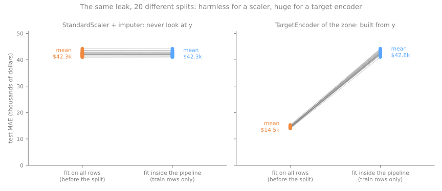
For the scaler, the leak changes the MAE by $4 on average, and by at most $96 in any split: the mean and standard deviation of 16,512 or of 20,640 districts are practically the same numbers, and the scaler never looks at the price. For the target encoder, the leak makes the error look $28,300 smaller on average, and at least $27,100 smaller in every split. The rule that follows is not "scalers are safe". It is: you cannot know the size of a leak without measuring both versions, and with every fitted step inside the pipeline there is nothing to measure. The more a step uses the target (target encoding, feature selection, oversampling), the bigger the potential leak; the cross-validation and data leakage lesson measures more of them.
One column is enough to see why the scaler barely leaked on a random split and when it would stop being harmless. The simulator fits the lesson's two steps (median imputation, then the scaler) on a column with holes, in one of two ways: on the training rows only (as the pipeline does) or on all rows before the split. Compare the two modes on a random split; then switch the test set to a later period in which prices rose.
On a random split the test rows look like the training rows, so adding them to the fit barely changes the statistics: that is the small scaler leak measured above. When the test set comes from a later period, the leaked mean and standard deviation already contain the new prices: the shift looks smaller than it is, and the filled holes land a little closer to the truth (a median resists a minority of high values). Nothing about the model improved; only the evaluation did. Inside the pipeline, the test rows never take part in a fit, whatever the split.
Looking ahead: tuning through the pipeline
Every setting of every step is reachable from the outside with a double-underscore path, step__parameter, nested as deep as the pipeline is (columntransformer__num__simpleimputer__strategy). get_params lists them, and set_params changes any of them without rebuilding the pipeline:
params = full.get_params()
print(len(params), "parameters, e.g.:")
for name in params:
    if name.endswith(('n_neighbors', 'strategy', 'handle_unknown')):
        print("  ", name, "=", params[name])
full.set_params(kneighborsregressor__n_neighbors=20)
print(full[-1])
46 parameters, e.g.:
   columntransformer__num__simpleimputer__strategy = median
   columntransformer__cat__handle_unknown = ignore
   kneighborsregressor__n_neighbors = 10
KNeighborsRegressor(n_neighbors=20)
After set_params, the next fit uses the new value. This is what makes automatic tuning possible: a search tries several values of kneighborsregressor__n_neighbors or of columntransformer__num__simpleimputer__strategy, and since each try refits the whole pipeline, the preprocessing is re-learned for every candidate on the rows used for training, and never on the rows used for scoring. Choosing such values honestly requires scoring them on data that is neither the training set nor the test set; scikit-learn's GridSearchCV does it with the pipeline and these names, and it is the subject of the cross-validation lesson. Until then, one rule: never choose a setting by looking at the test score.
Design habit
Start every project by writing the pipeline skeleton, even before choosing the model. It forces the train/test discipline from the first line of code, the model can be swapped by changing one line, and the object you evaluate is exactly the object you will ship.
Exercises
- By hand. A column has training values 10, NaN, 30, 50 and new values NaN, 70. Compute the median, mean and standard deviation that
SimpleImputer(strategy='median')followed byStandardScaler()learn, and the two transformed new values. Check with a pipeline. Then compute whatfit_transformon the two new rows would give. - Bug 1 with another scaler. Repeat the regional-batch experiment of bug 1 with
MinMaxScalerinstead ofStandardScaler, in both the model and the bug. Is the damage larger or smaller? Which statistic of a batch does min–max re-learn, and why is it more fragile than a mean? - Ratios as a step. Rooms per household, bedrooms per room and people per household are more meaningful than raw counts. Write them as a
FunctionTransformer(use a function that receives a DataFrame and returns one with the three new columns, andfeature_names_outas a function that returns their names), put it in the numeric branch, and compare the test MAE with the lesson's $41,552. - The size of a leak. Repeat the target-encoding experiment with zones rounded to one decimal (about 10 km) instead of two. How many zones have a single district now? Does the gap between the leaky and the honest MAE grow or shrink, and why?
Lab: from raw Titanic rows to a saved model
The preprocessing handout ended with a ColumnTransformer that turns the 891 raw Titanic passengers into a matrix of numbers, without training any model. This lab finishes the job: the same kind of preprocessing, now in a pipeline with a model at the end, fit on training rows, evaluated once on the test rows, opened up to check what it learned, used on new raw passengers, saved to disk and extended with a transformer of your own. The model is again a black box, a k-NN classifier with its default settings (it predicts "survived" when most of the 5 most similar training passengers survived; see k-NN).
Run the blocks in order, in one session. Every output below is what the code prints. To work on it directly, download the lab notebook and open it in Jupyter or Colab (File → Upload notebook).
Step 1 — load and look
import numpy as np
import pandas as pd

url = "https://raw.githubusercontent.com/hsandmann/biblio/refs/heads/main/ml/aula04/titanic/train.csv"
df = pd.read_csv(url)
print(df.shape)
print("missing:", df.isna().sum()[lambda s: s > 0].to_dict())
print(df[['Name', 'Sex', 'Age', 'Fare', 'Cabin', 'Embarked']].head(3).to_string())
(891, 12)
missing: {'Age': 177, 'Cabin': 687, 'Embarked': 2}
                                                  Name     Sex   Age     Fare Cabin Embarked
0                              Braund, Mr. Owen Harris    male  22.0   7.2500   NaN        S
1  Cumings, Mrs. John Bradley (Florence Briggs Thayer)  female  38.0  71.2833   C85        C
2                               Heikkinen, Miss. Laina  female  26.0   7.9250   NaN        S
891 passengers and 12 columns: identifiers (PassengerId, Name, Ticket), numbers (Age, SibSp, Parch, Fare), categories stored as text or as numbers (Sex, Embarked, Pclass), the cabin and the target Survived. Three columns have holes: Age in 177 rows (20%), Cabin in 687 (77%) and Embarked in 2. The first three rows already show everything the preprocessing must handle: text, NaN, and fares on a skewed scale (7.25 against 71.28). Nothing is cleaned by hand. The pipeline receives this table as it is, now and in production.
Step 2 — split once
from sklearn.model_selection import train_test_split

X = df.drop(columns='Survived')              # all 11 raw columns, text and holes included
y = df['Survived']
X_train, X_test, y_train, y_test = train_test_split(X, y, test_size=0.2, stratify=y, random_state=42)
print(X_train.shape, X_test.shape)
print(f"survival rate: train {y_train.mean():.3f} · test {y_test.mean():.3f}")
712 passengers to train, 179 to test, both with a survival rate of about 38% thanks to stratify. X keeps all 11 raw columns, including those the model will not use: deciding what to use is the pipeline's job, so the table given to it at prediction time can be the same raw table. The test rows are not touched until the score of step 4.
Step 3 — the preprocessing, column by column
from sklearn.compose import ColumnTransformer
from sklearn.impute import SimpleImputer
from sklearn.neighbors import KNeighborsClassifier
from sklearn.pipeline import Pipeline, make_pipeline
from sklearn.preprocessing import FunctionTransformer, OneHotEncoder, StandardScaler

preprocess = ColumnTransformer([
    ('num',  make_pipeline(SimpleImputer(strategy='median'), StandardScaler()),
             ['Age', 'SibSp', 'Parch']),
    ('fare', make_pipeline(SimpleImputer(strategy='median'),
                           FunctionTransformer(np.log1p, feature_names_out='one-to-one'),
                           StandardScaler()),
             ['Fare']),
    ('cat',  make_pipeline(SimpleImputer(strategy='most_frequent'),
                           OneHotEncoder(handle_unknown='ignore', sparse_output=False)),
             ['Pclass', 'Sex', 'Embarked']),
])
model = Pipeline([('prep', preprocess), ('knn', KNeighborsClassifier())])

used = [c for _, _, cols in preprocess.transformers for c in cols]
for name, _, cols in preprocess.transformers:
    print(f"{name:4s} <- {cols}")
print("dropped by remainder='drop':", [c for c in X.columns if c not in used])
num  <- ['Age', 'SibSp', 'Parch']
fare <- ['Fare']
cat  <- ['Pclass', 'Sex', 'Embarked']
dropped by remainder='drop': ['PassengerId', 'Name', 'Ticket', 'Cabin']
Three branches, as in the handout: numbers get the median and the scaler; the fare, which is very skewed, gets the median, then \(\log(1 + x)\), then the scaler; the categories get the most frequent value and one-hot encoding (Pclass is treated as a category, with no assumption that 2nd class is "halfway" between 1st and 3rd). The loop prints the routing. The four columns that no branch mentions are dropped by remainder='drop': the three identifiers and Cabin. They are in X, and they will never reach the model. Nothing has been fit yet: model is a recipe. In Jupyter, a cell containing just model draws it as a diagram.
Step 4 — fit on train, score on test
from sklearn.dummy import DummyClassifier

model.fit(X_train, y_train)
baseline = DummyClassifier(strategy='most_frequent').fit(X_train, y_train)
print(f"test accuracy · pipeline {model.score(X_test, y_test):.3f} · "
      f"always 'did not survive' {baseline.score(X_test, y_test):.3f}")
One call to fit fits three imputers, two scalers, the logarithm step, the encoder and the classifier, in the right order, all on the 712 training passengers. On the 179 test passengers the pipeline is right 78.2% of the time, against 61.5% for a "model" that always answers the majority class. There was nothing to tune (the classifier keeps its default settings), so the test set is used once, here.
Step 5 — what each step learned
prep = model.named_steps['prep']
num_imputer, num_scaler = prep.named_transformers_['num']
print("Age, SibSp, Parch medians:", num_imputer.statistics_)
print("means after imputing:     ", num_scaler.mean_.round(3))
print("standard deviations:      ", num_scaler.scale_.round(3))
print("rows the scaler saw:      ", num_scaler.n_samples_seen_)
print("Age median, train only vs all 891 rows:", X_train['Age'].median(), "vs", X['Age'].median())
fare_imputer, _, fare_scaler = prep.named_transformers_['fare']
print(f"Fare: median {fare_imputer.statistics_[0]:.2f} · mean of log1p(Fare) {fare_scaler.mean_[0]:.3f}")
print("categories:", [c.tolist() for c in prep.named_transformers_['cat'][-1].categories_])
Age, SibSp, Parch medians: [28.5  0.   0. ]
means after imputing:      [29.556  0.493  0.39 ]
standard deviations:       [13.016  1.06   0.838]
rows the scaler saw:       712.0
Age median, train only vs all 891 rows: 28.5 vs 28.0
Fare: median 14.45 · mean of log1p(Fare) 2.951
categories: [[1, 2, 3], ['female', 'male'], ['C', 'Q', 'S']]
Every learned value can be read, and each one is proof of where it was learned:
- The age median is 28.5, not 28.0. 28.0 is the median of all 891 passengers; 28.5 is the median of the 712 training passengers. The imputer never saw the test rows.
n_samples_seen_confirms it for the scaler: 712. - The scaler learned from imputed values. The mean age, 29.556, is the mean of the training ages after the holes were filled with 28.5, because the pipeline fits each step on the output of the previous one.
- The fare branch learned in its own units. Its imputer learned a median fare of £14.45, and its scaler learned the mean of \(\log(1 + \text{fare})\), 2.951, because the scaler sits after the logarithm.
- The encoder learned three lists of categories. Any other value at prediction time is "unknown" (step 7).
Step 6 — what the model sees
names = prep.get_feature_names_out()
print(len(names), "columns reach the model:", list(names))
prep.set_output(transform='pandas')
print(prep.transform(X_test.head(3)).round(2).T)
12 columns reach the model: ['num__Age', 'num__SibSp', 'num__Parch', 'fare__Fare', 'cat__Pclass_1', 'cat__Pclass_2', 'cat__Pclass_3', 'cat__Sex_female', 'cat__Sex_male', 'cat__Embarked_C', 'cat__Embarked_Q', 'cat__Embarked_S']
                  565   160   553
num__Age        -0.43  1.11 -0.58
num__SibSp       1.42 -0.47 -0.47
num__Parch      -0.47  0.73 -0.47
fare__Fare       0.28 -0.11 -0.86
cat__Pclass_1    0.00  0.00  0.00
cat__Pclass_2    0.00  0.00  0.00
cat__Pclass_3    1.00  1.00  1.00
cat__Sex_female  0.00  0.00  0.00
cat__Sex_male    1.00  1.00  1.00
cat__Embarked_C  0.00  0.00  1.00
cat__Embarked_Q  0.00  0.00  0.00
cat__Embarked_S  1.00  1.00  0.00
12 columns reach the model: 3 numbers, the fare, and 3 + 2 + 3 one-hot columns. The three test passengers shown are all third-class men. A hand check with the numbers of step 5: the first passenger has two siblings or spouses aboard, \((2 - 0.493)/1.060 = 1.42\); the second travels with one parent or child, \((1 - 0.390)/0.838 = 0.73\); a passenger with no parents or children gets \((0 - 0.390)/0.838 = -0.47\). With set_output, every transformed value has a name and every row keeps its index (565, 160, 553), so any suspicious number can be traced back to the raw row.
Step 7 — new passengers, raw
new = pd.DataFrame({
    'PassengerId': [901, 902, 903], 'Pclass': [3, 1, 2],
    'Name': ['Doe, Mr. John', 'Roe, Mrs. Jane', 'Poe, Miss. Ann'],
    'Sex': ['male', 'female', 'female'], 'Age': [25, np.nan, 30],
    'SibSp': [0, 1, 0], 'Parch': [0, 0, 0], 'Ticket': ['A1', 'B2', 'C3'],
    'Fare': [8.05, 80.0, 15.0], 'Cabin': [np.nan, 'C85', np.nan],
    'Embarked': ['S', 'C', 'B'],             # 'B' (Belfast) never appears in the training data
})
print(prep.transform(new)[['num__Age', 'cat__Embarked_C', 'cat__Embarked_Q', 'cat__Embarked_S']].round(2))
print("P(survived):", model.predict_proba(new)[:, 1].round(2), "· prediction:", model.predict(new))
   num__Age  cat__Embarked_C  cat__Embarked_Q  cat__Embarked_S
0     -0.35              0.0              0.0              1.0
1     -0.08              1.0              0.0              0.0
2      0.03              0.0              0.0              0.0
P(survived): [0. 1. 1.] · prediction: [0 1 1]
Three invented passengers, in the raw format of the original table: 11 columns, text included, one missing age and one port that does not exist in the data. The pipeline does not care about the columns it drops (Name, Ticket, Cabin), fills the missing age of the second passenger with the training median, \((28.5 - 29.556)/13.016 = -0.08\), and gives the third, who boarded at "B", zeros in the three Embarked columns instead of an error. The probabilities are the fraction of survivors among the 5 nearest training passengers, so they move in steps of 0.2; here the neighbors are unanimous: the third-class man did not survive, the two women did.
Step 8 — save, load, compare
import os
import joblib

joblib.dump(model, 'titanic-knn.joblib')
loaded = joblib.load('titanic-knn.joblib')
print(f"{os.path.getsize('titanic-knn.joblib') / 1e3:.0f} kB")
print("same test predictions:", np.array_equal(loaded.predict(X_test), model.predict(X_test)))
print("same probabilities for the new rows:",
      np.array_equal(loaded.predict_proba(new), model.predict_proba(new)))
The file holds the whole chain (imputers, scalers, encoder and classifier, with everything they learned) in 162 kB, most of it the 712 training passengers that k-NN keeps. Loaded back, it gives the same predictions and the same probabilities, to the last digit, from the same raw rows. That file is what a service would load to answer requests. Loading it requires a compatible version of scikit-learn, and loading a file from someone you do not trust is a security risk: both are discussed in MLOps.
Step 9 — a transformer of your own: the title
from sklearn.base import BaseEstimator, TransformerMixin

class TitleExtractor(TransformerMixin, BaseEstimator):
    """Name -> title ('Mr', 'Mrs', ...); titles rarer than min_count in TRAIN become 'Rare'."""
    def __init__(self, min_count=10):
        self.min_count = min_count

    def _titles(self, X):
        names = pd.Series(np.asarray(X).ravel())
        return names.str.extract(r',\s*([^.]+)\.')[0].str.strip()

    def fit(self, X, y=None):
        counts = self._titles(X).value_counts()
        self.titles_ = sorted(counts[counts >= self.min_count].index)   # learned on train
        return self

    def transform(self, X):
        t = self._titles(X)
        return t.where(t.isin(self.titles_), 'Rare').to_frame('title')

    def get_feature_names_out(self, input_features=None):
        return np.array(['title'])

prep2 = ColumnTransformer(preprocess.transformers + [
    ('title', make_pipeline(TitleExtractor(), OneHotEncoder(handle_unknown='ignore', sparse_output=False)),
     ['Name'])])
model2 = Pipeline([('prep', prep2), ('knn', KNeighborsClassifier())]).fit(X_train, y_train)
print("titles learned on train:", model2['prep'].named_transformers_['title'][0].titles_)
print("titles of the new rows: ", TitleExtractor().fit(X_train[['Name']]).transform(new[['Name']])['title'].to_list())
print(f"test accuracy · without title {model.score(X_test, y_test):.3f} · with title {model2.score(X_test, y_test):.3f}")
titles learned on train: ['Master', 'Miss', 'Mr', 'Mrs']
titles of the new rows:  ['Mr', 'Mrs', 'Miss']
test accuracy · without title 0.782 · with title 0.816
TitleExtractor has something to learn, so it is a class and not a FunctionTransformer: in fit it counts the titles of the training passengers and keeps those with at least 10 (Master, Miss, Mr, Mrs); in transform, every other title (Dr, Rev, Col, ...) becomes 'Rare'. A title that was frequent only in the test set would be 'Rare' too, which is the honest behavior. get_feature_names_out lets the encoder that follows name its columns. The new branch is added to the three existing ones, and the accuracy goes from 78.2% to 81.6%: "Master" marks boys, and "Miss" often young unmarried women, so the title carries age information even for passengers whose age is missing. A caveat: 3.4 points on 179 passengers is 6 passengers. Deciding to keep the title because of this number would be a decision taken on the test set; the honest way is a validation split (exercise 2 below) or the cross-validation you will meet later.
Your turn
- The deck. The first letter of
Cabinis the deck (A to G, T), and a missing cabin is information too (mostly third class). Add a branch that turnsCabininto the deck, with'U'for missing, followed by one-hot encoding. Write the conversion first as alambdainside aFunctionTransformer, fit, and tryjoblib.dumpon the model. What happens, and why does a function defined withdeffix it? - Choose
khonestly. Carve a validation split out ofX_train(25% of it, stratified). Forkin 1, 5, 15, 45, usemodel.set_params(knn__n_neighbors=k), fit on the rest of the training rows and score on the validation rows. Pick the bestk, refit on all ofX_train, and only then look at the test accuracy, once. (The cross-validation lesson will make this choice more robust.) - Break it on purpose. Predict on
X_testwith its columns in reverse order; onX_test.to_numpy(); and onX_test.drop(columns='Cabin'). Which of the three work, which fail, and what in the pipeline explains each result? - Clip the fare. Replace
log1pin the'fare'branch with the lesson'sClipper(percentiles 1 and 99). Print itsupper_and compare it with the largest fare in the training rows. Does the test accuracy change? Would you expect k-NN to be more sensitive to the fare's outliers than a model that only compares a value to a threshold?
References
- Buitinck, L.; Louppe, G.; Blondel, M.; Pedregosa, F.; Mueller, A.; Grisel, O.; Niculae, V.; Prettenhofer, P.; Gramfort, A.; Grobler, J.; Layton, R.; VanderPlas, J.; Joly, A.; Holt, B.; Varoquaux, G. "API design for machine learning software: experiences from the scikit-learn project." ECML PKDD Workshop: Languages for Data Mining and Machine Learning (2013): 108–122 — the estimator, transformer and pipeline interfaces used in this lesson, and why they look the way they do. arXiv
- Pedregosa, F.; Varoquaux, G.; Gramfort, A.; Michel, V.; Thirion, B.; Grisel, O.; Blondel, M.; Prettenhofer, P.; Weiss, R.; Dubourg, V.; Vanderplas, J.; Passos, A.; Cournapeau, D.; Brucher, M.; Perrot, M.; Duchesnay, É. "Scikit-learn: Machine Learning in Python." Journal of Machine Learning Research 12 (2011): 2825–2830. full text
- Micci-Barreca, D. "A Preprocessing Scheme for High-Cardinality Categorical Attributes in Classification and Prediction Problems." ACM SIGKDD Explorations 3, no. 1 (2001): 27–32 — target encoding with smoothing, the method behind
TargetEncoder. DOI - Kaufman, S.; Rosset, S.; Perlich, C.; Stitelman, O. "Leakage in Data Mining: Formulation, Detection, and Avoidance." ACM TKDD 6, no. 4 (2012) — a taxonomy of leakage with real competition cases. DOI
- Sculley, D.; Holt, G.; Golovin, D.; Davydov, E.; Phillips, T.; Ebner, D.; Chaudhary, V.; Young, M.; Crespo, J.-F.; Dennison, D. "Hidden Technical Debt in Machine Learning Systems." Advances in Neural Information Processing Systems 28 (NeurIPS 2015): 2503–2511 — "pipeline jungles" and the cost of training code and serving code that drift apart. full text