Data Preprocessing

A learning algorithm receives a matrix of numbers and a cost function. It does not know that the Fare column of the Titanic is in 1912 pounds, that Sex has no order, or that 177 ages were simply never recorded. It minimizes the cost with the numbers you hand it, and if those numbers are badly prepared, it minimizes the wrong thing, with full confidence. Preprocessing turns raw columns into numbers an algorithm can use without being fooled. Three problems come up in almost every table:

This lesson treats them in that order: scaling, shape (skewed columns), encoding and imputation, each measured on small examples you can check with a calculator, then on the Titanic passenger list (891 passengers of the 1912 voyage, one row each). EDA was about looking at a table; this lesson is about changing it. One rule runs through all of it: every preprocessing step learns something from data (a mean, a median, a list of categories), and it must learn it from the training rows only. The next lesson, Pipelines, turns that rule into code that cannot be broken by accident.

No model is needed for any of this, and none has been taught yet. The only one that appears is a k-NN classifier at the end of the lab, used as a clearly labeled black box to show that preprocessing changes the results a model reports.

How this lesson is organized

The lesson has two approaches. Each has slides, text and a lab to do in class; the quiz at the end covers the fundamental one. Start with the fundamental approach: the advanced one builds on it.

Both labs use the same lab notebook: download it and open it in Jupyter or Colab (File → Upload notebook). The fundamental part runs from step 1 to 6, the advanced part from step 7 to 9.

Fundamental approach

One question drives this part: how do raw columns become numbers a model can use without being fooled? Every answer is measured first on a few numbers you can check with a calculator, then on the Titanic.

This part follows one path in five stages, drawn below: 1. scale, so that no column owns the distance because of its unit; 2. fit on train only, the rule every step obeys; 3. fix the shape of skewed columns, which a scaler cannot do; 4. encode categories as numbers without inventing an order; 5. impute the holes, after asking why they are there. Each stage links to its section, and in the slides a strip at the bottom shows which stage you are in.

Fundamental approach slides

Click the slides and use the ← → arrows to navigate; F opens full screen and Esc shows every slide. Open the slides in a new tab

1. Why scale features?

Three passengers, by hand

Stage 1. Take three real passengers from the Titanic list, described by two columns, age and fare:

import numpy as np
import pandas as pd

url = "https://raw.githubusercontent.com/hsandmann/biblio/refs/heads/main/ml/aula04/titanic/train.csv"
df = pd.read_csv(url)
trio = df.set_index('PassengerId').loc[[1, 117, 152], ['Name', 'Age', 'Fare']]
print(trio)

                                          Name   Age   Fare
PassengerId
1                      Braund, Mr. Owen Harris  22.0   7.25
117                       Connors, Mr. Patrick  70.5   7.75
152          Pears, Mrs. Thomas (Edith Wearne)  22.0  66.60

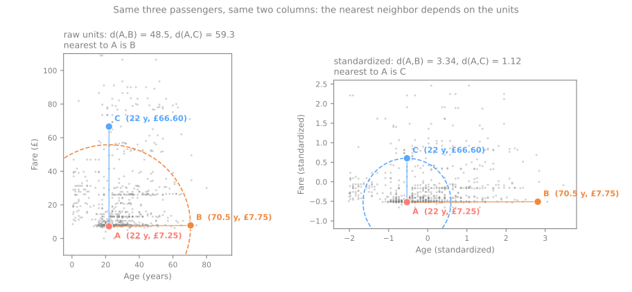
Call them A (a 22-year-old on a £7.25 third-class ticket), B (a 70.5-year-old with an equally cheap ticket) and C (a 22-year-old who paid £66.60 for first class). Which one is closest to A? The Euclidean distance adds up the squared differences, column by column:

In raw units, the 70-year-old is A's nearest neighbor, because a difference of 48.5 years is a smaller number than a difference of 59.35 pounds. Nothing says a year and a pound should weigh the same; that is just what happens when you subtract raw numbers. Now express each column in standard deviations instead of its unit: subtract the column mean and divide by the column standard deviation (\(z = (x - \mu)/\sigma\), computed over the 714 passengers whose age is known).

X = trio[['Age', 'Fare']].to_numpy()
dist = lambda a, b: np.sqrt(((a - b) ** 2).sum())
print(f"raw units:    d(A,B) = {dist(X[0], X[1]):.2f}   d(A,C) = {dist(X[0], X[2]):.2f}")

known = df.dropna(subset=['Age'])                         # the 714 passengers with an age
mu = known[['Age', 'Fare']].mean().to_numpy()
sd = known[['Age', 'Fare']].std(ddof=0).to_numpy()
Z = (X - mu) / sd
print(f"mean {mu.round(2)}   std {sd.round(2)}")
print(f"standardized: d(A,B) = {dist(Z[0], Z[1]):.2f}   d(A,C) = {dist(Z[0], Z[2]):.2f}")

raw units:    d(A,B) = 48.50   d(A,C) = 59.35
mean [29.7  34.69]   std [14.52 52.88]
standardized: d(A,B) = 3.34   d(A,C) = 1.12

With \(\sigma_{\text{Age}} = 14.52\) and \(\sigma_{\text{Fare}} = 52.88\), the 48.5-year gap between A and B is \(48.5 / 14.52 = 3.34\) standard deviations, while the £59.35 gap between A and C is only \(59.35 / 52.88 = 1.12\). After standardizing, C is the nearest neighbor, and the ranking flips (figure script):

Neither answer is "true": the raw one is an accident of the units, and the standardized one is a choice that gives each column the same say. The simulator makes the accident visible. It shows the same forty people and the same two columns; the only thing that changes is the unit printed on one of them.

Slide the unit from thousands to cents and watch the five nearest neighbors of the red point become a different five. Nothing about anyone changed. But k-NN would now return a different answer, k-means would find different clusters, and PCA would aim its first component at whichever column happens to carry bigger numbers. That is the precise sense in which distance-based methods are "sensitive to scale": the algorithm is not reading your features, it is reading their numerical magnitudes. Press standardize and the neighbor list stops depending on the unit at all.

Which column owns the distance?

The example is not a coincidence of three rows. For two rows drawn at random, the expected squared difference in a column is twice that column's variance, so each column's share of the average squared distance is its share of the total variance:

v = known[['Age', 'Fare', 'SibSp', 'Parch']].var(ddof=0)
print((100 * v / v.sum()).round(1))

Age       7.0
Fare     92.9
SibSp     0.0
Parch     0.0
dtype: float64

On raw Titanic columns, 92.9% of the distance between two passengers is fare difference, 7.0% is age, and the two family counts contribute nothing visible. A k-NN on raw columns is, in practice, a k-NN on fare. After standardizing, every column has variance 1, so each of the four gets 25%.

Which models care

• Distance-based methods: k-NN, k-means, kernel SVMs; the distance is dominated by the largest-scale feature.
• Variance-based methods: PCA finds directions of maximum variance, so the largest-scale feature wins by default.
• Gradient-based and penalized models: linear and logistic regression trained by gradient descent, neural networks, and Ridge/Lasso, whose penalty treats all coefficients as if their features were comparable.
• Trees do not care. Decision trees, random forests and gradient boosting split on one feature at a time ("is Age < 12?"). Any increasing transformation of a column moves the threshold but sends the same rows to each side.

2. Scaling methods

A scaler is a linear map applied to each column separately, \(x' = (x - \text{center}) / \text{spread}\). The four common ones differ only in which statistics they use for the center and the spread:

By hand, on a column with an outlier

Five households report a monthly income, in thousands of reais: 1, 2, 3, 4 and 40. The fifth is an outlier. The statistics each scaler needs, by hand (note that scikit-learn's standard deviation divides by \(n\), not \(n-1\)):

• mean \(\mu = (1+2+3+4+40)/5 = 10\); deviations \(-9, -8, -7, -6, 30\); \(\sigma = \sqrt{(81+64+49+36+900)/5} = \sqrt{226} = 15.03\);
• minimum 1, maximum 40, range 39;
• median 3; quartiles \(Q_1 = 2\), \(Q_3 = 4\), so IQR = 2;
• largest absolute value 40.

Applying the formulas to the first household (income 1): standard \((1-10)/15.03 = -0.599\); min-max \((1-1)/39 = 0\); robust \((1-3)/2 = -1\); max-abs \(1/40 = 0.025\). scikit-learn confirms the whole table:

from sklearn.preprocessing import MaxAbsScaler, MinMaxScaler, RobustScaler, StandardScaler

income = np.array([[1.], [2.], [3.], [4.], [40.]])       # R$ thousand; the last one is an outlier
table = pd.DataFrame({'raw': income.ravel()})
for scaler in [StandardScaler(), MinMaxScaler(), RobustScaler(), MaxAbsScaler()]:
    table[type(scaler).__name__] = scaler.fit_transform(income).ravel()
print(table.round(3))

std = StandardScaler().fit(income)
rob = RobustScaler().fit(income)
print("StandardScaler learned mean_", std.mean_, "scale_", std.scale_.round(3))
print("RobustScaler   learned center_", rob.center_, "scale_", rob.scale_)

    raw  StandardScaler  MinMaxScaler  RobustScaler  MaxAbsScaler
0   1.0          -0.599         0.000          -1.0         0.025
1   2.0          -0.532         0.026          -0.5         0.050
2   3.0          -0.466         0.051           0.0         0.075
3   4.0          -0.399         0.077           0.5         0.100
4  40.0           1.996         1.000          18.5         1.000
StandardScaler learned mean_ [10.] scale_ [15.033]
RobustScaler   learned center_ [3.] scale_ [2.]

The learned statistics are stored in the fitted object, in attributes whose names end with an underscore (mean_, scale_, center_): scikit-learn's convention for "learned from the data".

The simulator redoes the whole computation, one statistic or one row per step: the mean and the standard deviation, then each household's z-score and min-max value side by side, then the median and IQR of the robust scaler and the maximum of the max-abs one, every value placed on its scaler's axis. Before stepping, predict which axis will keep the four ordinary households apart.

Who sets the scale

Look at the four ordinary households in each column. Under StandardScaler they span \(-0.599\) to \(-0.399\), a width of 0.2; under MinMaxScaler and MaxAbsScaler, less than 0.08. The outlier sets the scale: it inflates \(\sigma\) (15.03, against 1.12 for the four ordinary values alone) and it is the maximum. Under RobustScaler, median and IQR come from the middle of the data, so the ordinary households keep a width of 1.5 and the outlier is left far away, at 18.5 (figure script):

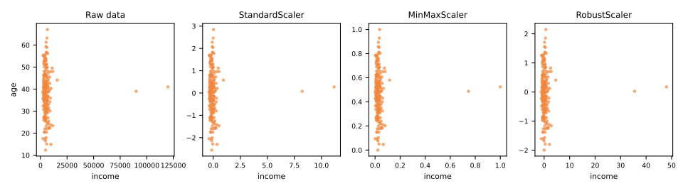
Inside a single column, every scaler keeps the same geometry: in all four versions the ordinary households occupy the same 8% of the column's range, because a linear map cannot change proportions. What changes is how large their differences are compared with the other columns, and that is what a distance adds up. If this income column sits next to an age column scaled to standard deviation 1, then under MinMaxScaler two ordinary households look almost identical in income, and age decides everything. RobustScaler keeps the ordinary spread at a size comparable to other robustly scaled columns.

Two warnings on names and neighbors. Normalization is ambiguous: in tabular ML it usually means min-max, in statistics it can mean "make it look normal", and scikit-learn's Normalizer is something else again: it rescales each row to unit length (used for text vectors), not each column. Say which one you mean, or write the formula. And a new value outside the training range leaves the promised interval: an income of 80 would become \((80-1)/39 = 2.03\) under the min-max scaler fitted above.

3. Fit on the training set, transform everything else

Stage 2. Every scaler above learned something: a mean, a standard deviation, a median, a range. Those are parameters of your model just as much as its weights are, so they obey the same rule as the weights: learn them on the training rows, then apply them, frozen, to every other row. In scikit-learn the two moments are separate methods: fit learns and stores, transform applies, and fit_transform does both on the same data.

A minimal example: the training set has five passengers aged 20 to 40; two new passengers, aged 60 and 70, arrive later.

train = np.array([[20.], [25.], [30.], [35.], [40.]])
test = np.array([[60.], [70.]])

scaler = StandardScaler().fit(train)
print("learned on train: mean", scaler.mean_, "std", scaler.scale_.round(2))
print("RIGHT  transform(test):        ", scaler.transform(test).ravel().round(2))
print("WRONG  fit_transform(test):    ", StandardScaler().fit_transform(test).ravel().round(2))
print("WRONG  fit_transform(one row): ", StandardScaler().fit_transform([[70.]]).ravel())
both = np.vstack([train, test])
print("WRONG  fit before the split: mean", both.mean().round(2), "std", both.std().round(2))

learned on train: mean [30.] std [7.07]
RIGHT  transform(test):         [4.24 5.66]
WRONG  fit_transform(test):     [-1.  1.]
WRONG  fit_transform(one row):  [0.]
WRONG  fit before the split: mean 40.0 std 17.11

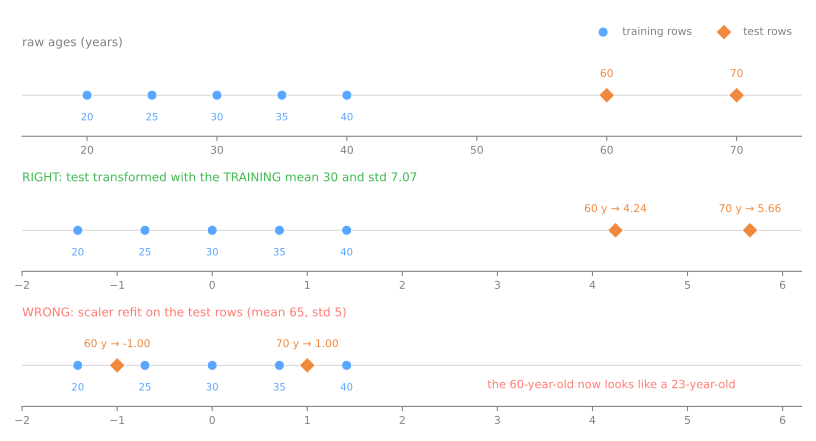
Read the four lines as four situations (figure script):

• Right. With the training mean 30 and standard deviation 7.07, the 60-year-old becomes \((60-30)/7.07 = 4.24\): "far older than anyone seen in training", which is the truth.
• Refitting on the test set. A new scaler fitted on the two test rows uses their mean (65) and spread (5), and maps them to \(-1\) and \(+1\). In the training set, \(-1\) meant \(30 - 7.07 = 22.9\) years. The 60-year-old is now encoded as a 23-year-old, and whatever the model learned about 23-year-olds is applied to him.
• Refitting on a single row. In production, predictions often arrive one at a time. A scaler fitted on one row maps every value to 0, the mean of that row: every passenger becomes "perfectly average".
• Fitting before the split. Fitting on all seven rows gives mean 40 and standard deviation 17.11; the test rows have influenced the numbers used to transform the training rows. This one does not produce an absurd value. It leaks: information from the test set reaches training, and the evaluation becomes optimistic.

The simulator goes through the four situations with the arithmetic in view: what each call of the scaler learns, and where the two new passengers land on the scaled axis. Predict, before each step, whether the 60-year-old will still look older than everyone in training.

How much the leak costs depends on what the step learns. For a scaler on hundreds of rows, often almost nothing: the cross-validation lesson measures it at 97.9% both ways. For a step that looks at the target, such as the target encoding of section 11, it can manufacture accuracy from nothing. Rather than judging each case, make the rule impossible to break: Pipelines bundle every step with the model so that a single fit touches only training rows.

4. Skewed features

Stage 3. A scaler shifts and stretches the axis; it cannot change the shape of a distribution. The Titanic fares have a long right tail: half the tickets cost less than £14.46, and three cost £512. The skewness you met in EDA summarizes that asymmetry: it is the average of the cubed z-scores, \(\frac{1}{n}\sum z_i^3\) (pandas applies a small-sample correction). It is 0 for a symmetric distribution, positive when the long tail is on the right.

fare = df[['Fare']]
print(f"zero fares: {(fare['Fare'] == 0).sum()}   median: {fare['Fare'].median()}   max: {fare['Fare'].max()}")
print(f"skewness raw            {fare['Fare'].skew():.2f}")
print(f"skewness standardized   {pd.Series(StandardScaler().fit_transform(fare).ravel()).skew():.2f}")
print(f"skewness sqrt           {np.sqrt(fare['Fare']).skew():.2f}")
print(f"skewness log1p          {np.log1p(fare['Fare']).skew():.2f}")

zero fares: 15   median: 14.4542   max: 512.3292
skewness raw            4.79
skewness standardized   4.79
skewness sqrt           2.09
skewness log1p          0.39

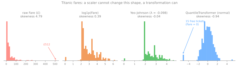
The raw skewness is 4.79, and standardizing leaves it at exactly 4.79, as it must. A nonlinear transformation is needed:

• log, \(x' = \log x\), compresses the right tail: multiplications become additions, so £8 → £80 and £50 → £500 become equal steps. Prices, incomes and populations often look roughly normal on a log scale. The Titanic has 15 free tickets, and \(\log 0 = -\infty\), so the practical version is \(\log(1 + x)\), np.log1p. It brings the skewness from 4.79 to 0.39.
• square root is a milder compression, often used for counts. Here it only gets to 2.09.

A few things to keep in mind:

• Check after transforming. A transformation is a hypothesis, not a recipe: the only way to know that the log was a good idea is to recompute the skewness (or look at the histogram) afterwards.
• Order: shape, then scale. Take the log first and standardize the logged column. Scaling first and then taking a log would undo the scaling, and would fail on the negative values the scaler created.
• Who cares: linear models and anything that computes distances or means. Trees do not: the log is increasing, so it sends the same rows to each side of any threshold.

Choosing the power by hand, as here, is a sound first move. The advanced approach lets the data choose it.

5. Encoding categorical features

Stage 4. Algorithms need numbers. A categorical column comes in three kinds, and each has its natural encoding:

• nominal: categories with no order (port of embarkation, color, city) → one-hot;
• ordinal: categories with a real order (ticket class 1st > 2nd > 3rd, education level, size S < M < L) → integers in that order;
• binary: two categories (Sex) → a single 0/1 column.

Integer codes invent distances

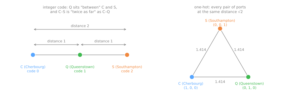
The tempting shortcut is to number the categories. OrdinalEncoder does exactly that, in alphabetical order: for the Titanic ports, Cherbourg = 0, Queenstown = 1, Southampton = 2. Any method that computes with these numbers now believes things nobody said:

from sklearn.metrics import pairwise_distances
from sklearn.preprocessing import OneHotEncoder, OrdinalEncoder

ports = pd.DataFrame({'Embarked': ['C', 'Q', 'S']})
codes = OrdinalEncoder().fit_transform(ports)
onehot = OneHotEncoder(sparse_output=False).fit_transform(ports)
print("integer codes:", codes.ravel())
print(pairwise_distances(codes))
print("one-hot rows:")
print(onehot)
print(pairwise_distances(onehot).round(3))

integer codes: [0. 1. 2.]
[[0. 1. 2.]
 [1. 0. 1.]
 [2. 1. 0.]]
one-hot rows:
[[1. 0. 0.]
 [0. 1. 0.]
 [0. 0. 1.]]
[[0.    1.414 1.414]
 [1.414 0.    1.414]
 [1.414 1.414 0.   ]]

With integer codes, Queenstown lies "between" Cherbourg and Southampton, and Cherbourg–Southampton is "twice as far" as Cherbourg–Queenstown. With one-hot encoding, each port gets its own column, and all three pairs sit at the same distance \(\sqrt{1^2 + 1^2} = 1.414\): no order, no preferred pair (figure script).

The simulator encodes the three ports one row at a time, first as integer codes and then as one-hot vectors, and computes every pairwise distance in both encodings. Predict the three one-hot distances before the step that computes them.

A linear model is misled in another way. It gives the integer column one coefficient, so the effect of going from code 0 to 1 is forced to equal the effect of going from 1 to 2. The survival rates by port show how false that is:

print(df.groupby('Embarked')['Survived'].mean().round(3))

Embarked
C    0.554
Q    0.390
S    0.337
Name: Survived, dtype: float64

From C to Q survival drops 16.4 points, from Q to S another 5.3; a single slope on the codes cannot represent both steps, and with another alphabet (or another language) the order of the codes would change and the slope with it. One-hot gives each port its own coefficient. Trees are the exception again: a tree can cut at 0.5 and then at 1.5, isolating each code in its own leaf, so integer codes are acceptable (and more compact) for tree models.

Ordinal encoding: you declare the order

When the order is real, integers are the right encoding, as long as you give the order. The alphabet does not know about education levels:

levels = pd.DataFrame({'education': ['high school', 'master', 'bachelor', 'high school']})
print(OrdinalEncoder().fit(levels).categories_)
enc = OrdinalEncoder(categories=[['high school', 'bachelor', 'master']])
print(enc.fit_transform(levels).ravel())

[array(['bachelor', 'high school', 'master'], dtype=object)]
[0. 2. 1. 0.]

By default the categories are sorted alphabetically, which puts high school between bachelor and master. With categories= stated explicitly, the codes follow the real order (0, 1, 2). The Titanic's Pclass is already stored as 1, 2, 3 in a meaningful order; treating it as ordinal (one column) or nominal (three one-hot columns) is a modeling choice: the ordinal version assumes that going from 1st to 2nd class matters as much as going from 2nd to 3rd.

One-hot: unseen categories

A fitted OneHotEncoder knows the categories it saw during fit, and by default it refuses any other one. Suppose the training rows only contain S, C and Q, and a passenger who boarded in Belfast (B) shows up later:

train_ports = pd.DataFrame({'Embarked': ['S', 'C', 'S', 'Q', 'S', 'C']})
new = pd.DataFrame({'Embarked': ['Q', 'B']})              # 'B' never appeared in training

enc = OneHotEncoder(sparse_output=False).fit(train_ports)
try:
    enc.transform(new)
except ValueError as e:
    print("default:", e)

enc = OneHotEncoder(sparse_output=False, handle_unknown='ignore').fit(train_ports)
print(enc.get_feature_names_out())
print(enc.transform(new))

default: Found unknown categories ['B'] in column 0 during transform
['Embarked_C' 'Embarked_Q' 'Embarked_S']
[[0. 1. 0.]
 [0. 0. 0.]]

With the default, a single unseen value crashes the prediction. With handle_unknown='ignore', the unknown port is encoded as all zeros, which honestly says "none of the categories I know". This is common in practice: a rare category may simply not land in the training split.

OneHotEncoder has a second option, drop='first', which removes one column per variable; section 10 shows which models need it.

6. Missing value imputation

Why is it missing?

Stage 5. The EDA lesson introduced the three mechanisms (Rubin, 1976). They decide what a fix can and cannot do:

print(df['Age'].isna().groupby(df['Pclass']).mean().round(3))
print(df.groupby(df['Age'].isna())['Survived'].mean().round(3))

Pclass
1    0.139
2    0.060
3    0.277
Name: Age, dtype: float64
Age
False    0.406
True     0.294
Name: Survived, dtype: float64

Age is missing for 27.7% of third-class passengers and 6.0% of second-class ones, which is evidence against MCAR. And those without a recorded age survived less often (29.4% against 40.6%). Both facts matter for the choice below.

Deleting rows or columns

dropna() removes every passenger with any missing value. It is acceptable only when very few rows are affected and the missingness is MCAR. For Age it would cost 177 rows (19.9%), and since the missing rows are concentrated in 3rd class, the remaining data would under-represent exactly the passengers who died most. Dropping a column is the right call when missingness is the rule rather than the exception, as for raw Cabin (77.1% missing), although even there the deck letter can be extracted and "unknown" kept as a category of its own.

Filling with one value shrinks the variance

SimpleImputer fills each column with one statistic learned on the training rows: mean, median (safer for skewed columns), most_frequent (the only one that works for text) or a constant (for example "unknown"). It is fast and simple, and it always does the same thing to the distribution: it piles every missing row on one value, which shrinks the spread. By hand, on six values of which two are missing:

from sklearn.impute import SimpleImputer

x = np.array([[2.], [4.], [np.nan], [6.], [np.nan], [8.]])
filled = SimpleImputer(strategy='mean').fit_transform(x)
print(filled.ravel())
print(f"variance of the 4 observed values: {np.nanvar(x):.3f}")
print(f"variance after mean imputation:    {filled.var():.3f}   ratio {filled.var() / np.nanvar(x):.3f}")

[2. 4. 5. 6. 5. 8.]
variance of the 4 observed values: 5.000
variance after mean imputation:    3.333   ratio 0.667

The observed values have mean 5 and variance \((9+1+1+9)/4 = 5\). The two imputed 5s add nothing to the sum of squared deviations but do add to the count, so the variance becomes \(20/6 = 3.33\): multiplied by \(4/6\), the fraction of observed values. That is a general law for mean imputation. On the Titanic, 714 of 891 ages are observed, so the standard deviation should shrink by \(\sqrt{713/890} = 0.895\) (with the \(n-1\) convention pandas uses):

age = df[['Age']]
filled = SimpleImputer(strategy='mean').fit_transform(age).ravel()
n_obs, n = age['Age'].notna().sum(), len(age)
print(f"std observed {age['Age'].std():.2f}   after mean imputation {filled.std(ddof=1):.2f}   "
      f"predicted {age['Age'].std() * np.sqrt((n_obs - 1) / (n - 1)):.2f}")

std observed 14.53   after mean imputation 13.00   predicted 13.00

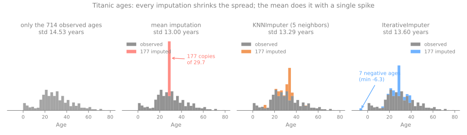
From 14.53 to 13.00 years, exactly as predicted. The model now believes ages are more homogeneous than they are, and 177 passengers share one invented age of 29.7.

The simulator repeats the six-value example step by step: what the imputer learns (fit), what it writes in the holes (transform) and why the variance falls to exactly 4/6 of its value. Its last step applies the same rule to the training ages of the lab. Predict the new variance before the step that computes it.

Keep the fact that it was missing

Imputation erases a piece of information: which values were invented. Yet on the Titanic, missing age goes with lower survival (29.4% against 40.6%). add_indicator=True appends a 0/1 column that records it, so a model can use the missingness itself:

imp = SimpleImputer(strategy='median', add_indicator=True)
out = imp.fit_transform(df[['Age']])
print(imp.get_feature_names_out())
print(out[[0, 5]])                                        # passenger 1 has an age, passenger 6 does not

['Age' 'missingindicator_Age']
[[22.  0.]
 [28.  1.]]

The flag costs one column, and it lets the model decide whether missingness is informative. For categorical columns, the equivalent is a category of its own (SimpleImputer(strategy='constant', fill_value='unknown')), which is often better than the mode.

7. Summary: preprocessing in six lines

1. Units decide distances by accident. Scale what distances, variances and penalties use; trees do not care.
2. Scalers differ in center and spread. Standard (mean, standard deviation), min-max (minimum, range), robust (median, IQR) and max-abs; an outlier sets the scale of all but the robust one.
3. Fit on train, transform everything else. Every step learns numbers, and it learns them from the training rows only.
4. A scaler cannot change the shape. A long right tail needs a nonlinear map such as log1p; check the skewness afterwards.
5. One-hot for nominal, declared order for ordinal. Integer codes invent distances; handle_unknown='ignore' keeps a new category from crashing the prediction.
6. Ask why it is missing; filling shrinks the spread. Mean or median imputation multiplies the variance by the observed fraction; add_indicator=True keeps the fact that a value was missing.

Fundamental lab — preparing the Titanic, column by column

The Titanic passenger list, from raw CSV to a numeric matrix with no holes, no text and comparable scales. Every choice is measured, and every statistic is learned on the training rows only. This part takes inventory, splits, asks why Age is missing, imputes it, encodes the categories and scales the numbers; bundling everything in one object and measuring what preprocessing changes in a model are left to the advanced lab.

Step 1 — load and take inventory

Predict. Before looking: which columns of a passenger list do you expect to have holes? Which ones are text, and which numbers are not really quantities?

import numpy as np
import pandas as pd

url = "https://raw.githubusercontent.com/hsandmann/biblio/refs/heads/main/ml/aula04/titanic/train.csv"
df = pd.read_csv(url)
print(df.shape)
inventory = pd.DataFrame({'numeric': [pd.api.types.is_numeric_dtype(df[c]) for c in df.columns],
                          'missing': df.isna().sum(),
                          'distinct': df.nunique()})
print(inventory)

(891, 12)
             numeric  missing  distinct
PassengerId     True        0       891
Survived        True        0         2
Pclass          True        0         3
Name           False        0       891
Sex            False        0         2
Age             True      177        88
SibSp           True        0         7
Parch           True        0         7
Ticket         False        0       681
Fare            True        0       248
Cabin          False      687       147
Embarked       False        2         3

891 passengers, 12 columns. The first task is to decide what each column is, which is not always what pandas stored:

• Survived is the target. It never enters the feature matrix.
• PassengerId is an identifier, a row number. Left in, a model could find meaningless cuts in it. It goes out.
• Age, SibSp, Parch and Fare are numeric quantities.
• Sex (binary), Embarked (nominal, 3 ports) and Pclass are categorical. Pclass is stored as a number (numeric: True), but 1, 2 and 3 are the labels of an ordered category, not a quantity.
• Name (891 distinct values), Ticket (681) and Cabin (147, and 687 missing) are near-identifiers: useless as they are, but hiding structure (a title, a deck). This lab leaves them out; the advanced Your turn extracts the title.

Three columns have holes: Age (177), Cabin (687) and Embarked (2).

Step 2 — split before anything else

Predict. The split comes before any imputation or scaling. What would go wrong if you computed the median age on all 891 passengers and only then split?

from sklearn.model_selection import train_test_split

features = ['Pclass', 'Sex', 'Age', 'SibSp', 'Parch', 'Fare', 'Embarked']
X, y = df[features], df['Survived']
X_train, X_test, y_train, y_test = train_test_split(X, y, test_size=0.2, stratify=y, random_state=42)
print(X_train.shape, X_test.shape)
print("missing in train:", X_train.isna().sum()[lambda s: s > 0].to_dict())
print("missing in test: ", X_test.isna().sum()[lambda s: s > 0].to_dict())

(712, 7) (179, 7)
missing in train: {'Age': 137, 'Embarked': 2}
missing in test:  {'Age': 40}

The split comes before any statistic is computed, because every step below learns something (a median, a mode, a mean and a standard deviation) and must learn it from the 712 training passengers only. It is the same split the logistic regression lab will use later: 20% for the test set, stratified on survival. The test set has 40 missing ages and no missing port; both missing Embarked values landed in the training rows.

Step 3 — why is Age missing?

Predict. Do you expect age to be missing equally often in the three classes? And would deleting the passengers without an age change what the training set looks like?

missing = X_train['Age'].isna()
print("share of missing Age by class:", missing.groupby(X_train['Pclass']).mean().round(3).to_dict())
print("survival rate, Age present / missing:", y_train.groupby(missing).mean().round(3).to_dict())
kept = X_train.dropna(subset=['Age'])
print(f"dropna keeps {len(kept)} of {len(X_train)} rows; "
      f"3rd-class share {(X_train['Pclass'] == 3).mean():.3f} -> {(kept['Pclass'] == 3).mean():.3f}")

share of missing Age by class: {1: 0.152, 2: 0.06, 3: 0.261}
survival rate, Age present / missing: {False: 0.405, True: 0.292}
dropna keeps 575 of 712 rows; 3rd-class share 0.549 -> 0.503

Looking only at the training rows: age is missing for 26.1% of third-class passengers, against 6.0% in second class and 15.2% in first. The missingness depends on an observed column, so it is not MCAR. It is also related to the outcome: 29.2% of the passengers without an age survived, against 40.5% of the others. Deleting those rows would keep 575 of the 712 passengers and shrink the share of third class from 54.9% to 50.3%: the training set would no longer look like the ship, and the missing-age signal would be gone. We impute instead, and keep the option of a missing flag (advanced Your turn, exercise 1).

Step 4 — compare imputation strategies for Age

Predict. After filling 137 holes with one value, will the standard deviation of the ages go up, stay the same or go down? Which age will become the most frequent one?

from sklearn.impute import SimpleImputer

cols = ['Age', 'Pclass', 'SibSp', 'Parch']
imputers = {'mean': SimpleImputer(strategy='mean'),
            'median': SimpleImputer(strategy='median')}
observed = X_train['Age'].dropna()
rows = {'observed only': [len(observed), observed.mean(), observed.std(), observed.min(),
                          observed.value_counts().iloc[0]]}
for name, imp in imputers.items():
    ages = pd.Series(imp.fit(X_train[cols]).transform(X_train[cols])[:, 0])
    rows[name] = [len(ages), ages.mean(), ages.std(), ages.min(), ages.value_counts().iloc[0]]
print(pd.DataFrame(rows, index=['n', 'mean', 'std', 'min', 'largest pile']).T.round(2))

                   n   mean    std   min  largest pile
observed only  575.0  29.81  14.49  0.42          26.0
mean           712.0  29.81  13.02  0.42         137.0
median         712.0  29.56  13.03  0.42         139.0

Each imputer is fitted on the training rows (fit) and applied to them (transform); the same fitted objects later transform the test rows, whose 40 missing ages receive the training mean or median, never a statistic of the test rows. How to read the table:

• observed only: the 575 real ages, standard deviation 14.49 years; the most frequent age (22) appears 26 times.
• mean and median: 137 passengers are stacked on a single value (29.81 or 28.5; the median pile has 139 because two real passengers are exactly 28.5), and the standard deviation falls to 13.02, which is \(14.49 \times \sqrt{574/711}\), the shrinkage law of section 6.

Neither recovers 14.49: filling with one value always shrinks the spread. For the rest of this lab we use the median, the simplest robust choice. Step 9, in the advanced lab, tries two imputers that look at the other columns.

Simulation: the shrinkage law, on holes you make. Take the 575 real ages of the training rows and erase 20%, 50% and 80% of them at random (MCAR). Fill the holes with the mean and compare the standard deviation with the law of section 6, the standard deviation of the kept ages times \(\sqrt{(n_{\text{kept}} - 1)/(n - 1)}\). Does the law hold every time? How far does the filled column drift from the 14.49 of the real ages?

rng = np.random.default_rng(0)
real = X_train['Age'].dropna()                                  # the 575 ages we do have
print(f"all 575 real ages: std {real.std():.2f}")
for erase in [0.2, 0.5, 0.8]:
    holed = real.copy()
    holed[rng.random(len(real)) < erase] = np.nan               # erase ages at random (MCAR)
    filled = SimpleImputer(strategy='mean').fit_transform(holed.to_frame()).ravel()
    n_kept = holed.notna().sum()
    law = holed.std() * np.sqrt((n_kept - 1) / (len(holed) - 1))
    print(f"erase {erase:.0%}: {n_kept} ages kept, std {holed.std():.2f} · after mean imputation "
          f"{filled.std(ddof=1):.2f} · law {law:.2f}")

all 575 real ages: std 14.49
erase 20%: 463 ages kept, std 14.65 · after mean imputation 13.15 · law 13.15
erase 50%: 285 ages kept, std 13.98 · after mean imputation 9.83 · law 9.83
erase 80%: 120 ages kept, std 13.62 · after mean imputation 6.20 · law 6.20

Step 5 — encode Sex, Embarked and Pclass

Predict. Three categorical columns with 2, 3 and 3 levels: how many one-hot columns will they become, and how many 1s will each row have?

from sklearn.preprocessing import OneHotEncoder

cat_cols = ['Sex', 'Embarked', 'Pclass']
cat_imp = SimpleImputer(strategy='most_frequent').set_output(transform='pandas')
cats_train = cat_imp.fit_transform(X_train[cat_cols])            # learns the modes on train
cats_test = cat_imp.transform(X_test[cat_cols])
print("modes learned on train:", cat_imp.statistics_)

ohe = OneHotEncoder(handle_unknown='ignore', sparse_output=False).fit(cats_train)
print(ohe.get_feature_names_out())
print(X_test[cat_cols].head(3).to_numpy().tolist())
print(ohe.transform(cats_test.head(3)))

modes learned on train: ['male' 'S' 3]
['Sex_female' 'Sex_male' 'Embarked_C' 'Embarked_Q' 'Embarked_S' 'Pclass_1'
 'Pclass_2' 'Pclass_3']
[['male', 'S', 3], ['male', 'S', 3], ['male', 'C', 3]]
[[0. 1. 0. 0. 1. 0. 0. 1.]
 [0. 1. 0. 0. 1. 0. 0. 1.]
 [0. 1. 1. 0. 0. 0. 0. 1.]]

The modes are learned on the training rows: male, S and 3, so the two missing ports become Southampton. One-hot encoding turns the 3 columns into 8 (2 sexes + 3 ports + 3 classes), named column_value. Each row has exactly three 1s, one per original column: the first test passenger is a man who boarded at Southampton in third class, and the third boarded at Cherbourg. Two choices were made here. Pclass is treated as nominal (three columns, no assumption that 2nd class sits exactly halfway between 1st and 3rd). And handle_unknown='ignore' means that a category never seen in training would be encoded as zeros instead of crashing the transform. There is no drop='first': the black-box model of step 8 computes distances, and for distances every category should keep its column.

Step 6 — scale the numeric columns

Predict. In raw units, which numeric column will own the distance between two passengers? And after scaling with the training statistics, will the test columns have mean exactly 0?

from sklearn.preprocessing import StandardScaler

num_cols = ['Age', 'SibSp', 'Parch', 'Fare']
num_imp = SimpleImputer(strategy='median').set_output(transform='pandas').fit(X_train[num_cols])
num_train, num_test = num_imp.transform(X_train[num_cols]), num_imp.transform(X_test[num_cols])
scaler = StandardScaler().set_output(transform='pandas').fit(num_train)
z_train, z_test = scaler.transform(num_train), scaler.transform(num_test)

share = lambda M: (100 * M.var() / M.var().sum()).round(1)     # share of the squared distance
print(pd.DataFrame({'raw %': share(num_train), 'scaled %': share(z_train)}))
print(pd.DataFrame({'train mean': z_train.mean(), 'train std': z_train.std(ddof=0),
                    'test mean': z_test.mean(), 'test std': z_test.std(ddof=0)}).round(3))

       raw %  scaled %
Age      6.8      25.0
SibSp    0.0      25.0
Parch    0.0      25.0
Fare    93.1      25.0
       train mean  train std  test mean  test std
Age           0.0        1.0     -0.036     0.995
SibSp        -0.0        1.0      0.141     1.178
Parch        -0.0        1.0     -0.053     0.791
Fare         -0.0        1.0      0.040     1.160

The first table is the lesson's variance argument on real data: in raw units, fare accounts for 93.1% of the squared distance between two passengers, age for 6.8%, and the family counts for nothing visible. After scaling, each column contributes 25%.

The second table is the fit-on-train rule made visible. On the training rows, every mean is 0 and every standard deviation is 1, by construction. On the test rows they are not: the means range from \(-0.053\) to 0.141 and the standard deviations from 0.791 to 1.178, because the test passengers were transformed with the training statistics. That imperfection is the correct result. If the test columns came out with mean exactly 0 and standard deviation exactly 1, the scaler would have been fitted on them.

Simulation: whose neighbors? Take the first test passenger and find the 5 training passengers closest to them on the four numeric columns, once in raw units (num_train, num_test) and once scaled (z_train, z_test). How many passengers appear in both lists? What do the neighbors of each list have in common?

from sklearn.metrics import pairwise_distances

first = X_test.index[0]                                         # the first test passenger
print("test passenger", first, num_test.loc[first].to_dict())
nearest = {}
for name, A, q in [('raw', num_train, num_test.loc[[first]]), ('scaled', z_train, z_test.loc[[first]])]:
    d = pairwise_distances(q, A).ravel()
    nearest[name] = A.index[np.argsort(d)[:5]]                  # the 5 nearest training passengers
    print(f"{name} units, 5 nearest:")
    print(num_train.loc[nearest[name]].to_string())
print("in both lists:", len(set(nearest['raw']) & set(nearest['scaled'])))

test passenger 565 {'Age': 24.0, 'SibSp': 2.0, 'Parch': 0.0, 'Fare': 24.15}
raw units, 5 nearest:
      Age  SibSp  Parch  Fare
316  24.0    1.0    0.0  26.0
600  24.0    2.0    1.0  27.0
312  26.0    1.0    1.0  26.0
551  27.0    0.0    0.0  26.0
874  28.0    1.0    0.0  24.0
scaled units, 5 nearest:
      Age  SibSp  Parch     Fare
330  28.5    2.0    0.0  23.2500
301  28.5    2.0    0.0  23.2500
48   28.5    2.0    0.0  21.6792
69   26.0    2.0    0.0   8.6625
392  28.0    2.0    0.0   7.9250
in both lists: 0

To close the fundamental part. In one sentence each: (1) why is a k-NN on raw Titanic columns, in practice, a k-NN on fare? (2) Where does the median of step 4 come from, and what do the test passengers' missing ages receive? (3) Why are the scaled test columns of step 6 not exactly mean 0 and standard deviation 1, and why is that correct?

Your turn (fundamental)

At home:

1. Another scaler. Redo step 6 with RobustScaler instead of StandardScaler. Print its scale_: which columns get a spread of exactly 1, and why, for each one? How do the shares of the squared distance change?
2. Fare's shape. Compute the skewness of X_train['Fare'], of np.log1p(X_train['Fare']) and of the logged column after a StandardScaler. Which step changes the shape, and which does not?
3. Pclass as ordinal. In step 5, leave Pclass out of the one-hot and keep it as a single column (1, 2, 3). How many columns does the encoding produce now, and what does this choice assume about the three classes?

Advanced approach

The fundamental part prepared each column with the simplest correct tool. This part asks what those tools miss, and how to choose among the alternatives: why gradient descent also wants scaled features, how to let the data choose a power transformation, why a linear model chokes on a full one-hot encoding, what to do with hundreds of categories without leaking the target, and how the other columns can fill a hole. The code blocks continue those of sections 1 to 6.

This part follows one path in five stages, drawn below: 1. scale for gradients; 2. choose the power; 3. encode for the model; 4. impute from the other columns; 5. assemble the recipe. Each stage links to its section, and in the slides a strip at the bottom shows which stage you are in.

Advanced approach slides

Click the slides and use the ← → arrows to navigate; F opens full screen and Esc shows every slide. Open the slides in a new tab

8. Scale and gradient descent

Stage 1. Scale matters for a second reason, which you will meet in Gradient Descent. Gradient descent walks downhill on a loss surface, and with a squared loss the curvature of that surface along each direction is set by the variance of the features. When one feature has much larger numbers than another, the bowl becomes a long, narrow valley: a learning rate small enough not to overshoot across the steep direction crawls along the flat one. The ratio of the largest to the smallest curvature measures how elongated the valley is:

A = known[['Age', 'Fare']].to_numpy()
for name, M in [('raw', A - A.mean(0)), ('standardized', (A - A.mean(0)) / A.std(0))]:
    curv = np.linalg.eigvalsh(M.T @ M / len(M))           # curvatures of a squared loss
    print(f"{name:13s} curvatures {curv.round(2)}   ratio {curv.max() / curv.min():.1f}")

raw           curvatures [ 208.62 2798.59]   ratio 13.4
standardized  curvatures [0.9 1.1]   ratio 1.2

With age and fare in their raw units the valley is 13.4 times more curved in one direction than in the other; after standardizing, the ratio is 1.2 (the remainder comes from the small correlation between age and fare). A nearly round bowl is what lets gradient descent use one learning rate for every weight.

9. Let the data choose the power

Stage 2. Section 4 chose the transformation by hand: a log or a square root. Instead of choosing the power by hand, Box-Cox (Box & Cox, 1964) estimates it from the data. It is a family indexed by \(\lambda\), \(x' = (x^\lambda - 1)/\lambda\), with \(\lambda = 0\) meaning \(\log x\), and PowerTransformer picks the \(\lambda\) that makes the result as close to normal as possible (by maximum likelihood). Box-Cox requires strictly positive values. Yeo-Johnson (Yeo & Johnson, 2000) extends the family to zero and negative values; for \(x \ge 0\) it is Box-Cox applied to \(x + 1\), so \(\lambda = 0\) is exactly log1p. QuantileTransformer goes further: it replaces each value by its rank (its quantile) and maps the rank onto a normal (or uniform) distribution, forcing any shape into the target one.

from sklearn.preprocessing import PowerTransformer, QuantileTransformer

try:
    PowerTransformer(method='box-cox').fit(fare)
except ValueError as e:
    print("Box-Cox on all fares:", e)
bc = PowerTransformer(method='box-cox', standardize=False).fit(fare[fare['Fare'] > 0])
print(f"Box-Cox on the 876 positive fares: lambda = {bc.lambdas_[0]:.3f}")

yj = PowerTransformer(method='yeo-johnson', standardize=False).fit(fare)
print(f"Yeo-Johnson: lambda = {yj.lambdas_[0]:.3f}   skewness {pd.Series(yj.transform(fare).ravel()).skew():.2f}")

qt = QuantileTransformer(n_quantiles=100, output_distribution='normal').fit(fare)
fare_q = qt.transform(fare).ravel()
print(f"Quantile (normal): skewness {pd.Series(fare_q).skew():.2f}   "
      f"the 15 free tickets all map to {fare_q.min():.2f}")

Box-Cox on all fares: The Box-Cox transformation can only be applied to strictly positive data
Box-Cox on the 876 positive fares: lambda = -0.524
Yeo-Johnson: lambda = -0.098   skewness -0.04
Quantile (normal): skewness -0.94   the 15 free tickets all map to -5.20

Box-Cox refuses the column outright because of the zero fares. Yeo-Johnson picks \(\lambda = -0.098\), close to 0, so the data essentially asked for a log (a slightly stronger one) and the skewness drops to \(-0.04\). The quantile transform is the most aggressive and still ends at \(-0.94\): ranks cannot separate ties, so the 15 free tickets pile up at \(-5.20\), the bottom of its range (figure script):

A few things to keep in mind:

• \(\lambda\) and the quantiles are learned, so power and quantile transforms follow the fit-on-train rule like any scaler. (Above we looked at the whole column, as in an EDA. In a model they are fitted on the training rows.)
• Shape, then scale, built in. PowerTransformer standardizes its output by default (standardize=True), for the reason given in section 4.
• The quantile transform keeps only the order. How far apart two fares were in pounds no longer matters, only how many passengers lie between them. It is useful for extremely irregular columns, and it should be used with care.

10. One-hot for linear models: the dropped column

Stage 3. Section 5 kept every one-hot column. Another option of OneHotEncoder, drop='first', removes one column per variable. Here is why it exists. In a full one-hot encoding, the columns of one variable always add up to 1 (every passenger embarked somewhere), which is exactly the constant column that a linear model's intercept multiplies:

full = OneHotEncoder(sparse_output=False).fit_transform(train_ports)
first = OneHotEncoder(sparse_output=False, drop='first').fit_transform(train_ports)
ones = np.ones((len(train_ports), 1))                     # the column the intercept multiplies
print("row sums of the full one-hot:", full.sum(axis=1))
print("rank of [intercept | full one-hot]  :", np.linalg.matrix_rank(np.hstack([ones, full])),
      "for", 1 + full.shape[1], "columns")
print("rank of [intercept | drop='first']  :", np.linalg.matrix_rank(np.hstack([ones, first])),
      "for", 1 + first.shape[1], "columns")

row sums of the full one-hot: [1. 1. 1. 1. 1. 1.]
rank of [intercept | full one-hot]  : 3 for 4 columns
rank of [intercept | drop='first']  : 3 for 3 columns

Four columns with rank 3 means one column is a combination of the others (intercept = C + Q + S): the weights of a linear model are then not unique, since adding 5 to the three port weights and subtracting 5 from the intercept gives the same predictions. Dropping one category (the first, C, becomes the reference) restores full rank, and each remaining coefficient then reads "compared with Cherbourg". The logistic regression lab, later in the course, uses exactly this. The rule of thumb:

• drop='first' for linear models with an intercept and no penalty, when you want to read the coefficients;
• keep all columns for trees, k-NN and regularized models: dropping a category makes the reference special (for a distance, "reference" and "unknown" become the same all-zeros vector).

11. High cardinality and target encoding

Ports and sexes have two or three levels. Tickets, cabins and names have hundreds, and one-hot stops being an option.

High cardinality

The number of distinct values decides what is reasonable:

for col in ['Sex', 'Embarked', 'Pclass', 'Cabin', 'Ticket', 'Name']:
    print(f"{col:9s} {df[col].nunique():4d} distinct values")

title = df['Name'].str.extract(r',\s*([^.]+)\.')[0].to_frame('title')
print(title['title'].value_counts().head(5).to_dict(), '...', title['title'].nunique(), 'titles')
enc = OneHotEncoder(min_frequency=10, sparse_output=False).fit(title)
print(enc.get_feature_names_out())

Sex          2 distinct values
Embarked     3 distinct values
Pclass       3 distinct values
Cabin      147 distinct values
Ticket     681 distinct values
Name       891 distinct values
{'Mr': 517, 'Miss': 182, 'Mrs': 125, 'Master': 40, 'Dr': 7} ... 17 titles
['title_Master' 'title_Miss' 'title_Mr' 'title_Mrs'
 'title_infrequent_sklearn']

With 2 or 3 levels, one-hot is trivial. One-hot on Ticket would create 681 columns of almost only zeros for 891 rows: more columns than information, and a guaranteed recipe for overfitting. Before encoding a high-cardinality column, look for the structure hidden inside it: the first letter of Cabin is the deck (8 levels), and Name contains a title (Mr, Miss, Mrs, Master, ...) that encodes sex, approximate age and marital status at once. Then group the rare levels: min_frequency=10 keeps the four titles that appear at least 10 times and merges the other 13 into a single infrequent column.

Target encoding, and why it leaks

For columns with hundreds of levels there is a more compact option: replace each category by the mean of the target in that category (Micci-Barreca, 2001). A ticket shared by three passengers of whom two survived becomes 0.667. It is one column, whatever the cardinality. It is also the most dangerous encoding in this lesson, because it is built from the target itself.

To see the danger, build a column with no information at all: 2,000 passengers, each with one of 800 random ticket numbers, and a survival label drawn by coin flip. Encode it with the naive per-category mean computed on the training rows, then check the simplest possible rule, "predict survived if the encoded value is above 0.5":

from sklearn.model_selection import train_test_split
from sklearn.preprocessing import TargetEncoder

rng = np.random.default_rng(0)
noise = pd.DataFrame({'ticket': rng.integers(0, 800, 2000).astype(str),   # 800 random tickets
                      'survived': rng.integers(0, 2, 2000)})             # coin flips
tr, te = train_test_split(noise, test_size=0.3, random_state=0)
rule = lambda enc, y: ((enc > 0.5) == y).mean()                          # "survived if > 0.5"

means = tr.groupby('ticket')['survived'].mean()                          # naive target encoding
naive_tr = tr['ticket'].map(means)
naive_te = te['ticket'].map(means).fillna(tr['survived'].mean())
print(f"naive:        train {rule(naive_tr, tr['survived']):.3f}   test {rule(naive_te, te['survived']):.3f}")

te_enc = TargetEncoder(random_state=0)
cf_tr = te_enc.fit_transform(tr[['ticket']], tr['survived']).ravel()     # cross-fitted
cf_te = te_enc.transform(te[['ticket']]).ravel()
print(f"cross-fitted: train {rule(cf_tr, tr['survived']):.3f}   test {rule(cf_te, te['survived']):.3f}")

naive:        train 0.775   test 0.505
cross-fitted: train 0.496   test 0.505

On pure noise, the naive encoding "explains" 77.5% of the training labels, and drops to chance (50.5%) on new rows. The mechanism: most tickets appear only once or twice, so a row's encoded value is mostly its own label. Any model trained on that column learns to read the answer, not to predict it. scikit-learn's TargetEncoder avoids this with cross-fitting: fit_transform splits the training rows into folds and encodes each fold with means computed on the other folds, so no row ever sees its own label; it also shrinks the mean of rare categories toward the global mean. Its training score is at chance, as it should be.

Two rules follow. Never compute a target encoding on data that includes the rows you evaluate on. And use it through fit_transform on the training set (which cross-fits), then transform on the test set. The cross-validation lesson treats this family of mistakes in general. Two other compact options, without the target: frequency encoding (replace a category by how often it appears) and hashing (a fixed number of columns, collisions accepted).

12. Imputing from the other columns

Stage 4. Section 6 filled every hole with one value. Under MAR, the other columns carry information about the missing value, and two imputers use it:

• KNNImputer (Troyanskaya et al., 2001) finds the \(k\) rows most similar to the incomplete one, measuring distance only on the columns both rows have, and averages their values. Since it computes distances, it needs comparable scales, exactly like k-NN.
• IterativeImputer models each incomplete column as a regression on the others, fills it with the predictions, and cycles over the columns a few times. It is scikit-learn's version of the MICE procedure (van Buuren & Groothuis-Oudshoorn, 2011), still flagged as experimental, so it needs an extra import.

KNNImputer by hand, on five real passengers, one of whom (Mr. James Moran, fare £8.46) has no age:

from sklearn.impute import KNNImputer

toy = df.loc[[0, 1, 2, 3, 5], ['Age', 'Fare']]
print(toy)
print("KNNImputer (k=2):", KNNImputer(n_neighbors=2).fit_transform(toy)[-1])
print("mean imputation: ", SimpleImputer(strategy='mean').fit_transform(toy)[-1])

    Age     Fare
0  22.0   7.2500
1  38.0  71.2833
2  26.0   7.9250
3  35.0  53.1000
5   NaN   8.4583
KNNImputer (k=2): [24.      8.4583]
mean imputation:  [30.25    8.4583]

The fare differences from £8.46 are 1.2, 62.8, 0.5 and 44.6, so the two nearest passengers are those who paid £7.925 and £7.25, aged 26 and 22; their average, 24, is the imputed age. The mean imputer ignores the fare and answers 30.25. (Here only one column is available for the distance, so its scale does not matter; with several columns, it would.)

On the whole column, using class, siblings and parents as the other columns:

from sklearn.experimental import enable_iterative_imputer  # noqa: F401  (unlocks IterativeImputer)
from sklearn.impute import IterativeImputer

cols = df[['Age', 'Pclass', 'SibSp', 'Parch']]
for name, imp in [('KNNImputer', KNNImputer(n_neighbors=5)),
                  ('IterativeImputer', IterativeImputer(random_state=0)),
                  ('Iterative, min_value=0', IterativeImputer(random_state=0, min_value=0))]:
    ages = imp.fit_transform(cols)[:, 0]
    print(f"{name:23s} std {ages.std(ddof=1):.2f}   min {ages.min():6.2f}   negative ages {(ages < 0).sum()}")

KNNImputer              std 13.29   min   0.42   negative ages 0
IterativeImputer        std 13.60   min  -6.26   negative ages 7
Iterative, min_value=0  std 13.48   min   0.00   negative ages 0

Both spread the imputed values instead of stacking them (standard deviation 13.29 and 13.60, against 13.00 for the mean and 14.53 for the observed ages), because a passenger with three siblings in 3rd class gets a younger guess than a lone 1st-class traveler. No imputer recovers the original spread: the information was lost at collection time. And the regression-based imputer produced 7 negative ages, all for the children of one family traveling with 8 siblings: the regression extends the trend "more siblings, younger passenger" past zero, because it does not know that age is positive. min_value=0 removes the impossible values, but only by clipping them: those 7 passengers are now imputed as newborns. A regression on class and family counts is a crude model of age, and checking the imputed values is part of the job (figure script).

13. The preprocessing map

Stage 5. Everything together, column by column. Per column, in this order: missing values → shape → scale. The scaler should learn its statistics from the column as the model will receive it, holes filled and shape corrected; a log applied after scaling would undo the scaling (and fail on the negative values). Every step is fitted on the training rows only.

Which families care about which step:

Advanced lab — one object, a black-box model and smarter imputers

The fundamental lab built the matrix with four separately fitted objects. This part bundles them into one, uses a k-NN classifier as a black box (the k-NN lesson comes later in the course) to show that preprocessing changes the result a model reports, and tries the imputers that use the other columns. Continue in the same notebook, in the same session: the steps below use X_train, X_test, num_cols, cat_cols, cols and rows from steps 1 to 6.

Step 7 — everything in one object: a ColumnTransformer preview

Predict. Steps 5 and 6 used four fitted objects. Bundled into one, how many columns will the output have, and will any NaN be left in the test rows?

from sklearn.compose import ColumnTransformer
from sklearn.pipeline import make_pipeline

preprocess = ColumnTransformer([
    ('num', make_pipeline(SimpleImputer(strategy='median'), StandardScaler()), num_cols),
    ('cat', make_pipeline(SimpleImputer(strategy='most_frequent'),
                          OneHotEncoder(handle_unknown='ignore')), cat_cols)])
M_train = preprocess.fit_transform(X_train)       # every statistic is learned here, on train only
M_test = preprocess.transform(X_test)             # ... and only applied here
print(M_train.shape, M_test.shape, "NaN left in test:", int(np.isnan(M_test).sum()))
print(preprocess.get_feature_names_out())
print(M_test[:2].round(2))

(712, 12) (179, 12) NaN left in test: 0
['num__Age' 'num__SibSp' 'num__Parch' 'num__Fare' 'cat__Sex_female'
 'cat__Sex_male' 'cat__Embarked_C' 'cat__Embarked_Q' 'cat__Embarked_S'
 'cat__Pclass_1' 'cat__Pclass_2' 'cat__Pclass_3']
[[-0.43  1.42 -0.47 -0.16  0.    1.    0.    0.    1.    0.    0.    1.  ]
 [ 1.11 -0.47  0.73 -0.33  0.    1.    0.    0.    1.    0.    0.    1.  ]]

Steps 5 and 6 needed four fitted objects (two imputers, an encoder and a scaler), and every one of them had to be fitted on the right rows. A ColumnTransformer routes each list of columns through its own chain (median then scaling for the numbers; mode then one-hot for the categories) and puts the results side by side. One call to fit_transform on the training rows learns every statistic; transform applies all of them to the test rows. The result has 12 columns (4 numeric + 8 one-hot), no NaN and no text, and the names carry the branch that produced them (num__, cat__). The first test passenger is the same as in step 5: num__Age = \(-0.43\) (a little younger than the average passenger), then the one-hot block 0 1 | 0 0 1 | 0 0 1: male, Southampton, third class.

This is a preview. The next lesson covers Pipeline and ColumnTransformer properly: how to attach a model at the end, inspect every fitted step, and let cross-validation refit the whole chain in every fold.

Step 8 — does it matter? A black-box k-NN with and without scaling

Predict. The baseline that always answers "did not survive" gets 61.5%. Will a k-NN on unscaled columns be far above it? How much will scaling add?

from sklearn.dummy import DummyClassifier
from sklearn.neighbors import KNeighborsClassifier
from sklearn.preprocessing import MinMaxScaler, RobustScaler

baseline = DummyClassifier(strategy='most_frequent').fit(X_train, y_train)
print(f"baseline (always 'did not survive')   test accuracy {baseline.score(X_test, y_test):.3f}")
for name, scaler in [('no scaling', 'passthrough'), ('StandardScaler', StandardScaler()),
                     ('MinMaxScaler', MinMaxScaler()), ('RobustScaler', RobustScaler())]:
    prep = ColumnTransformer([
        ('num', make_pipeline(SimpleImputer(strategy='median'), scaler), num_cols),
        ('cat', make_pipeline(SimpleImputer(strategy='most_frequent'),
                              OneHotEncoder(handle_unknown='ignore')), cat_cols)])
    knn = make_pipeline(prep, KNeighborsClassifier(n_neighbors=5)).fit(X_train, y_train)
    print(f"k-NN (black box), {name:15s}     test accuracy {knn.score(X_test, y_test):.3f}")

baseline (always 'did not survive')   test accuracy 0.615
k-NN (black box), no scaling          test accuracy 0.676
k-NN (black box), StandardScaler      test accuracy 0.821
k-NN (black box), MinMaxScaler        test accuracy 0.804
k-NN (black box), RobustScaler        test accuracy 0.771

The classifier is a black box here: a k-NN predicts the outcome of a passenger by a vote among the 5 training passengers closest to them (the k-NN lesson explains it later in the course). The only thing that changes between the four lines is the scaler of the numeric columns; data, imputation, encoding and model are identical.

• The baseline that always answers "did not survive" gets 61.5% of the test passengers right. Any model has to beat that.
• Without scaling, k-NN reaches 67.6%, barely above the baseline: its neighbors are chosen almost only by fare (93.1% of the distance, step 6), and the sex and class columns, worth 0 or 1, hardly count.
• With StandardScaler, 82.1%: 14.5 points more, with the same model and the same data.
• MinMaxScaler gives 80.4% and RobustScaler 77.1%. The robust scaler leaves the extremes far away, as designed: fitted on these training rows, a £512 fare becomes 21.5 and 8 siblings becomes 8, while one-hot columns stay at 0 or 1, so a few extreme passengers are again dominated by fare and family size.

Two cautions. With 179 test passengers, each one is worth 0.56 points, so the differences between scalers (a few passengers) are not a reliable ranking; choosing among them is done on validation data or with cross-validation, never by trying several versions on the test set, as done here only to illustrate. The difference between scaling and not scaling, on the other hand, is large and repeats with other random splits.

Simulation: shape before scale. Fare is the most skewed column. Give it a branch of its own in the column transformer: median, then FunctionTransformer(np.log1p), then StandardScaler, with the other numeric columns in the usual branch. Does the skewness of the training fares drop? Does the k-NN of step 8 improve?

from sklearn.preprocessing import FunctionTransformer

rest = ['Age', 'SibSp', 'Parch']
logfare = ColumnTransformer([
    ('num', make_pipeline(SimpleImputer(strategy='median'), StandardScaler()), rest),
    ('fare', make_pipeline(SimpleImputer(strategy='median'), FunctionTransformer(np.log1p),
                           StandardScaler()), ['Fare']),                 # shape, then scale
    ('cat', make_pipeline(SimpleImputer(strategy='most_frequent'),
                          OneHotEncoder(handle_unknown='ignore')), cat_cols)])
knn_log = make_pipeline(logfare, KNeighborsClassifier(n_neighbors=5)).fit(X_train, y_train)
fares = num_train['Fare']
print(f"skewness of the training fares: raw {fares.skew():.2f} · log1p {np.log1p(fares).skew():.2f}")
print("share of the squared distance, log1p(Fare) unscaled:",
      share(num_train.assign(Fare=np.log1p(fares))).to_dict())
print(f"k-NN, log1p(Fare) then StandardScaler   test accuracy {knn_log.score(X_test, y_test):.3f}")

skewness of the training fares: raw 4.65 · log1p 0.31
share of the squared distance, log1p(Fare) unscaled: {'Age': 98.4, 'SibSp': 0.7, 'Parch': 0.4, 'Fare': 0.6}
k-NN, log1p(Fare) then StandardScaler   test accuracy 0.782

Step 9 — imputers that use the other columns

Predict. An imputer that looks at class and family size: will its imputed ages spread more or less than the median's? Can it produce an impossible age?

Step 4 compared imputers that use one value. Section 12 introduced two that use the other columns; this step fits both on the training rows and adds them to the same table (cols and rows come from step 4):

from sklearn.experimental import enable_iterative_imputer  # noqa: F401
from sklearn.impute import IterativeImputer, KNNImputer

others = {'knn': KNNImputer(n_neighbors=5),
          'iterative': IterativeImputer(random_state=0, min_value=0)}
for name, imp in others.items():
    ages = pd.Series(imp.fit(X_train[cols]).transform(X_train[cols])[:, 0])
    rows[name] = [len(ages), ages.mean(), ages.std(), ages.min(), ages.value_counts().iloc[0]]
print(pd.DataFrame(rows, index=['n', 'mean', 'std', 'min', 'largest pile']).T.round(2))

                   n   mean    std   min  largest pile
observed only  575.0  29.81  14.49  0.42          26.0
mean           712.0  29.81  13.02  0.42         137.0
median         712.0  29.56  13.03  0.42         139.0
knn            712.0  29.99  13.36  0.42          75.0
iterative      712.0  29.54  13.46  0.00          75.0

• knn and iterative use class and family counts, so the imputed ages vary from passenger to passenger and the spread shrinks less than with the mean or the median (13.36 and 13.46, against 13.02). Their largest pile is 75: many incomplete passengers have identical class and family counts, so they receive identical imputations. With min_value=0, the iterative imputer no longer produces negative ages, but its minimum of 0.00 says that some passengers were clipped to newborns.

None of them recovers 14.49. Which one leads to a better model can only be measured with a model and a validation procedure.

Simulation: a smarter imputer inside the pipeline. In the numeric branch of the step-8 pipeline (with StandardScaler), replace the median by KNNImputer(n_neighbors=5), once on raw units and once between two scalers (the imputer measures distances, so section 12 says it needs comparable scales). Does the k-NN's test accuracy improve?

branches = {'median, then scale': make_pipeline(SimpleImputer(strategy='median'), StandardScaler()),
            'KNNImputer on raw units, then scale': make_pipeline(KNNImputer(n_neighbors=5),
                                                                 StandardScaler()),
            'scale, KNNImputer, scale again': make_pipeline(StandardScaler(), KNNImputer(n_neighbors=5),
                                                            StandardScaler())}
for name, branch in branches.items():
    ct = ColumnTransformer([('num', branch, num_cols),
                            ('cat', make_pipeline(SimpleImputer(strategy='most_frequent'),
                                                  OneHotEncoder(handle_unknown='ignore')), cat_cols)])
    model = make_pipeline(ct, KNeighborsClassifier(n_neighbors=5)).fit(X_train, y_train)
    print(f"{name:37s} test accuracy {model.score(X_test, y_test):.3f}")

median, then scale                    test accuracy 0.821
KNNImputer on raw units, then scale   test accuracy 0.810
scale, KNNImputer, scale again        test accuracy 0.799

To close the lesson. In one sentence each: (1) what does a ColumnTransformer guarantee that four separately fitted objects do not? (2) Why can a log that fixes the shape of the fare still make the k-NN worse? (3) Why does an imputer that keeps more of the spread not necessarily give a better model?

Your turn (advanced)

At home, with more time:

1. The missing flag. Use SimpleImputer(strategy='median', add_indicator=True) in the numeric branch. How many columns does the output have now, and what is the name of the new one? Does the k-NN of step 8 change?
2. Titles. Extract the title from Name (df['Name'].str.extract(r',\s*([^.]+)\.')), add it to the features and to cat_cols, and encode it with OneHotEncoder(handle_unknown='ignore', min_frequency=10). Then impute Age with the median age of each title, learned on the training rows (groupby('Title')['Age'].median()). What does it give to the boys titled Master whose age is missing (3 of them in the training rows), compared with the global median of 28.5?
3. The leak, in numbers. Fit preprocess on all 891 rows instead of X_train. Compare the learned median age and the fare mean and standard deviation (preprocess.named_transformers_['num']) with the train-only version. Which statistic moves most, and why is that the one that depends on a few extreme rows?

Class materials

References

• Box, G. E. P.; Cox, D. R. "An Analysis of Transformations." Journal of the Royal Statistical Society B 26, no. 2 (1964): 211–252 — the Box-Cox family and the choice of \(\lambda\) by maximum likelihood. DOI
• Yeo, I.-K.; Johnson, R. A. "A New Family of Power Transformations to Improve Normality or Symmetry." Biometrika 87, no. 4 (2000): 954–959 — the extension to zero and negative values. DOI
• Rubin, D. B. "Inference and Missing Data." Biometrika 63, no. 3 (1976): 581–592 — the MCAR / MAR / MNAR distinction. DOI
• Troyanskaya, O. et al. "Missing Value Estimation Methods for DNA Microarrays." Bioinformatics 17, no. 6 (2001): 520–525 — k-nearest-neighbor imputation. DOI
• van Buuren, S.; Groothuis-Oudshoorn, K. "mice: Multivariate Imputation by Chained Equations in R." Journal of Statistical Software 45, no. 3 (2011): 1–67 — the chained-equations procedure behind IterativeImputer. DOI
• Micci-Barreca, D. "A Preprocessing Scheme for High-Cardinality Categorical Attributes in Classification and Prediction Problems." ACM SIGKDD Explorations Newsletter 3, no. 1 (2001): 27–32 — target encoding with shrinkage toward the global mean. DOI
• scikit-learn developers. "Preprocessing data" and "Imputation of missing values", scikit-learn User Guide. Preprocessing · Imputation

Quiz

The quiz covers the fundamental approach.