Machine Learning · Insper

Data Preprocessing

Advanced approach

What the simple recipes miss, and how to choose among the alternatives

The path of this part

Scale for gradientsthe curvature of the loss; one learning rate
Choose the powerBox-Cox, Yeo-Johnson, quantiles
Encode for the modelthe dropped column; hundreds of levels; target encoding
Impute from the other columnsKNNImputer, IterativeImputer; check the values
Assemble the recipethe map, column by column

Each stage answers one question: why does gradient descent want scaled features? → which power does a skewed column need? → what does each model need from a category? → can the other columns fill a hole? → what recipe does each column get?

Stage 1 · why does gradient descent want scaled features?

A long valley or a round bowl

With a squared loss, the curvature along each direction is set by the variance of the features: the eigenvalues of \(M^\top M / n\), with \(M\) the centered (age, fare) matrix of \(n\) rows.

raw	208.62, 2798.59	ratio 13.4
standardized	0.9, 1.1	ratio 1.2

A learning rate safe for the steep direction crawls along the flat one.

Standardized, the bowl is nearly round: gradient descent can use one learning rate for every weight (the gradient descent lesson).

Stage 2 · which power does a skewed column need?

Let the data choose the power

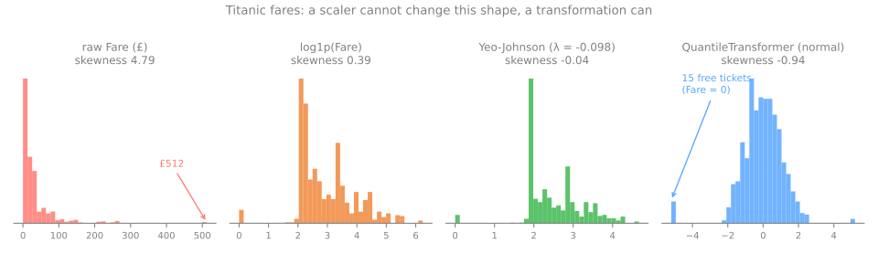
Fare skewness: 4.79 raw, 0.39 after log1p, −0.04 after Yeo-Johnson, −0.94 after QuantileTransformer

Box-Cox

\(x' = (x^\lambda - 1)/\lambda\), \(\lambda = 0\) means \(\log x\); \(\lambda\) by maximum likelihood. Needs \(x > 0\): refuses the 15 free tickets.

Yeo-Johnson

accepts zero and negatives. \(\lambda = -0.098\), close to a log → skewness −0.04.

QuantileTransformer

replaces each value by its rank → −0.94; the 15 free tickets pile up at −5.20.

\(\lambda\) and the quantiles are learned: fit on train. PowerTransformer standardizes its output by default (shape, then scale). Quantiles keep only the order.

Stage 3 · what does each model need from a category?

One-hot and the intercept: the dropped column

port	intercept	C	Q	S	C + Q + S
S	1	0	0	1	1
C	1	1	0	0	1
S	1	0	0	1	1
Q	1	0	1	0	1
S	1	0	0	1	1
C	1	1	0	0	1

The three port columns always add up to the intercept's column: rank 3 for 4 columns.

The weights are not unique: add 5 to the three port weights, subtract 5 from the intercept, same predictions.

drop='first' removes C, the reference: rank 3 for 3 columns, each coefficient reads "compared with Cherbourg".

drop='first' for linear models with an intercept and no penalty. Keep every column for trees, k-NN (k nearest neighbors) and regularized models: for a distance, "reference" and "unknown" would both be 0 0.

High cardinality, and target encoding

Ticket has 681 distinct values for 891 rows: one-hot would create 681 columns of almost only zeros, a recipe for overfitting.

First look for the structure inside: the deck letter of Cabin, the title in Name (Mr, Miss, Mrs, Master...).
Then group rare levels: min_frequency=10 keeps 4 titles and merges the other 13.
Target encoding: replace each category by the mean of the target in it. One column, whatever the cardinality.

Predict. A column with no information: 2,000 passengers, 800 random tickets, survival by coin flip. Encode it with the per-ticket mean, then apply "survived if > 0.5". What training accuracy do you expect?

Target encoding leaks

encoding of pure noise	train	test
naive per-category mean	0.775	0.505
`TargetEncoder` (cross-fitted)	0.496	0.505

Most tickets appear once or twice, so a row's encoded value is mostly its own label: the model learns to read the answer, not to predict it.
Cross-fitting: fit_transform encodes each fold with means from the other folds, so no row sees its own label; rare categories are shrunk toward the global mean.

Never compute a target encoding on rows you evaluate on: fit_transform on train, transform on test. Target-free options: frequency encoding, hashing.

Stage 4 · can the other columns fill a hole?

`KNNImputer`, by hand

Mr. James Moran paid £8.46 and has no age. The imputer looks for the \(k = 2\) passengers with the closest fare and averages their ages.

passenger	age	fare	\|fare − 8.46\|
3	26	£7.93	0.5
1	22	£7.25	1.2
4	35	£53.10	44.6
2	38	£71.28	62.8

Imputed age \((26 + 22)/2 = \mathbf{24}\). The mean imputer ignores the fare and answers 30.25. With several columns, the distance needs comparable scales, exactly like k-NN.

Imputing from the other columns

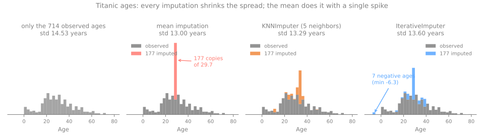
Std of Age: 14.53 observed, 13.00 mean imputation, 13.29 KNN, 13.60 iterative with 7 negative ages

`KNNImputer`

average of the \(k\) most similar rows. On class, siblings and parents: std 13.29, no impossible age.

`IterativeImputer`

a regression of each column on the others, cycled (MICE, multivariate imputation by chained equations). It produced 7 negative ages: it does not know that age is positive.

Both spread the guesses (13.29, 13.60 against 13.00 for the mean), but none recovers 14.53. Check the imputed values.

Stage 5 · what recipe does each column get?

The preprocessing map

Per column: missing values → shape → scale, every step fitted on the training rows. Click the answers to build a recipe.

Which families care about which step

model family	scaling	shape	encoding	missing values
k-NN, k-means, SVM, PCA	required	helps	one-hot	must be imputed
linear/logistic regression, neural networks	required	helps	one-hot, `drop='first'` if no penalty	must be imputed
trees, random forests, gradient boosting	not needed	not needed	ordinal codes are fine	scikit-learn's trees accept `NaN`

SVM: support vector machine; PCA: principal component analysis; NaN: not a number, a missing value.

A log applied after scaling would undo the scaling (and fail on negative values): shape before scale.

Summary

Scaling also makes the loss round: one learning rate for every weight.
Let the data choose the power: Yeo-Johnson accepts zeros; \(\lambda\) is learned on train.
drop='first' only for linear models with an intercept and no penalty.
Hundreds of levels: structure, rare levels grouped, cross-fitted target encoding.
Imputers that use the other columns spread the guesses; check what they invent.

Next: Pipelines, which make "fit on train, transform the rest" impossible to break by accident.

Advanced lab · about 25 min, in pairs

One object, a black-box model and smarter imputers: steps 7 to 9

Step 7: every statistic in one ColumnTransformer: 12 columns, no NaN, no text.
Step 8: a k-NN used as a black box, with and without scaling. Step 9: imputers that use the other columns.
Continue in the lab notebook, in the same session.
Simulations: shape before scale (step 8) and a smarter imputer inside the pipeline (step 9).

Predict. The baseline "always did not survive" gets 61.5%. A black-box k-NN with and without scaling, same data: how far apart?

Pace: step 7 in 5 min; step 8 and the first simulation in 10 min; step 9 and the second in 10 min.