The algorithm only sees numbers
It minimizes the cost with the numbers you hand it. If they are badly prepared, it minimizes the wrong thing, with full confidence.
incompatible scales
the column with the biggest numbers dominates distances and penalties
Fare 0 to 512, SibSp 0 to 8
text
there is no arithmetic with "female"
Sex, Embarked, Cabin, Ticket, Name
holes
most implementations refuse NaN
Age missing for 19.9%, Cabin for 77.1%
The plan: scaling → shape → encoding → imputation, each measured on a small example, then on the Titanic (891 passengers of the 1912 voyage). EDA looked at the table; this lesson changes it.
The path of this lesson
- Scaleunits decide distances; four scalers
- Fit on train onlyfit once on the training rows, transform the rest
- Fix the shapelog, Box-Cox, Yeo-Johnson
- Encode categoriesordinal, one-hot, target encoding
- Impute the holeswhy it is missing; one value, other columns, an indicator
Three passengers, by hand
| passenger | age | fare | |
|---|---|---|---|
| A | Braund, Mr. Owen Harris (3rd class) | 22.0 | £7.25 |
| B | Connors, Mr. Patrick | 70.5 | £7.75 |
| C | Pears, Mrs. Thomas (1st class) | 22.0 | £66.60 |
In raw units, the 70-year-old wins
| pair | age difference | fare difference | distance |
|---|---|---|---|
| A–B | 48.5 years | £0.50 | \(\sqrt{48.5^2 + 0.5^2} = 48.50\) |
| A–C | 0 years | £59.35 | \(\sqrt{0^2 + 59.35^2} = 59.35\) |
48.5 years is a smaller number than 59.35 pounds. Nothing says a year and a pound should weigh the same: it is just what happens when you subtract raw numbers.
Standardized, the ranking flips
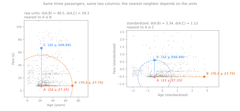
A–B: \(48.5 / 14.52 = \mathbf{3.34}\) std
A–C: \(59.35 / 52.88 = \mathbf{1.12}\) std
\(\mu\) and \(\sigma\) computed over the 714 passengers whose age is known.
Simulator: the unit decides the neighbors
Predict. Slide the income unit from thousands to cents. Do the 5 nearest neighbors of the red point stay the same? Then press standardize.
Which column owns the distance?
For two random rows, the expected squared difference in a column is twice its variance: each column's share of the distance is its share of the total variance.
share of the squared distance (raw)
Fare | 92.9% |
Age | 7.0% |
SibSp, Parch | 0.0% |
A k-NN on raw columns is, in practice, a k-NN on fare. Standardized: 25% each.
a forward look: gradient descent
With a squared loss, the curvature along each direction is set by the variance of the features. Age and fare:
| raw | 208.62, 2798.59 | ratio 13.4 |
| standardized | 0.9, 1.1 | ratio 1.2 |
A long narrow valley: a learning rate safe for the steep direction crawls along the flat one.
Which models care about scale
care
- distance-based: k-NN, k-means, kernel SVMs
- variance-based: PCA (the largest-scale feature wins by default)
- gradient-based and penalized: linear and logistic regression, neural networks, Ridge/Lasso
do not care
Trees, random forests, gradient boosting: they split on one feature at a time ("is Age < 12?").
Any increasing transformation moves the threshold but sends the same rows to each side.
Four scalers: \(x' = (x - \text{center}) / \text{spread}\)
| scaler | formula | center | spread | result |
|---|---|---|---|---|
StandardScaler | \((x - \mu) / \sigma\) | mean | standard deviation | mean 0, std 1 |
MinMaxScaler | \((x - x_{\min}) / (x_{\max} - x_{\min})\) | minimum | range | values in \([0, 1]\) |
RobustScaler | \((x - \text{median}) / \text{IQR}\) | median | IQR \(= Q_3 - Q_1\) | median 0, IQR 1 |
MaxAbsScaler | \(x / \max \lvert x \rvert\) | none (0 stays 0) | largest \(\lvert x \rvert\) | values in \([-1, 1]\) |
By hand: a column with an outlier
Five households, monthly income in R$ thousand: 1, 2, 3, 4 and 40.
- mean \(\mu = 10\); \(\sigma = \sqrt{(81+64+49+36+900)/5} = \sqrt{226} = 15.03\) (scikit-learn divides by \(n\))
- minimum 1, maximum 40, range 39
- median 3; \(Q_1 = 2\), \(Q_3 = 4\), so IQR = 2
First household (income 1): standard \((1-10)/15.03 = -0.599\) · min-max \(0\) · robust \((1-3)/2 = -1\) · max-abs \(1/40 = 0.025\)
The outlier sets the scale
| raw | Standard | MinMax | Robust | MaxAbs |
|---|---|---|---|---|
| 1 | −0.599 | 0.000 | −1.0 | 0.025 |
| 2 | −0.532 | 0.026 | −0.5 | 0.050 |
| 3 | −0.466 | 0.051 | 0.0 | 0.075 |
| 4 | −0.399 | 0.077 | 0.5 | 0.100 |
| 40 | 1.996 | 1.000 | 18.5 | 1.000 |
Width of the four ordinary values:
- Standard: 0.2 (the outlier inflates \(\sigma\): 15.03 against 1.12 without it)
- MinMax, MaxAbs: < 0.08 (the outlier is the maximum)
- Robust: 1.5, and the outlier is left far away, at 18.5
Learned statistics live in attributes ending with an underscore: mean_, scale_, center_.
Same geometry, different weight next to other columns
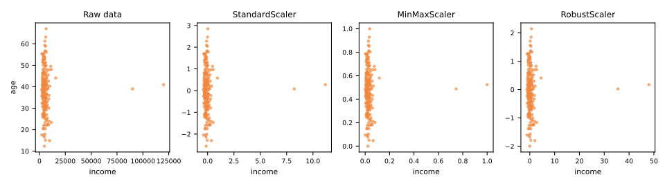
Inside the column the ordinary households always occupy the same 8% of the range: a linear map cannot change proportions. What changes is how big their differences are compared with the other columns, and that is what a distance adds up.
MinMaxScaler, next to an age column with std 1, two ordinary households look almost identical in income, and age decides everything.Choosing a scaler
| scaler | effect of outliers | typical use |
|---|---|---|
StandardScaler | moderate: they inflate \(\sigma\) | the default: linear models, SVM, PCA, neural networks |
MinMaxScaler | strong: one extreme value compresses the rest | a bounded range is required (pixel intensities) |
RobustScaler | weak: they are simply left far away | columns with outliers you decided to keep |
MaxAbsScaler | strong, like min-max | sparse data: zeros stay zeros |
- Normalization is ambiguous (min-max? "make it normal"? scikit-learn's
Normalizerrescales each row). Write the formula. - A new value outside the training range leaves the interval: an income of 80 becomes \((80-1)/39 = 2.03\) under min-max.
Fit on the training set, transform everything else
A mean or a standard deviation is a parameter of your model, just like a weight. fit learns and stores, transform applies, fit_transform does both on the same data.
training ages
20, 25, 30, 35, 40
mean 30, std 7.07
new passengers
60 and 70
StandardScaler().fit_transform(test) on the two new rows. What values do 60 and 70 receive?Four situations
| what the code does | 60 and 70 become | what went wrong |
|---|---|---|
right: transform(test) | \((60-30)/7.07 = 4.24\), 5.66 | nothing: "far older than anyone in training" |
| refit on the 2 test rows | −1, +1 (their mean 65, spread 5) | −1 meant 22.9 years: the 60-year-old is now 23 |
| refit on a single row | 0 | every passenger is "perfectly average" |
| fit before the split | learned: mean 40, std 17.11 | it leaks: the evaluation becomes optimistic |
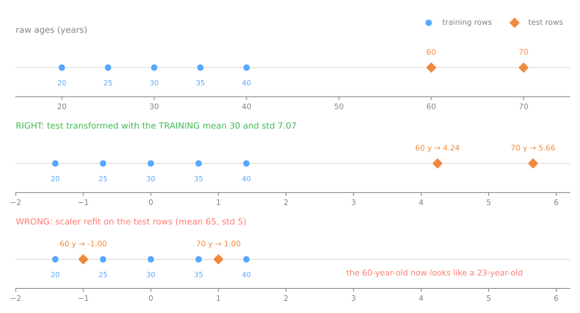
fit once, on the training rows. Validation, test and production only ever see transform.Skewed features: a scaler cannot change the shape
Titanic fares: half cost less than £14.46, three cost £512, and 15 tickets were free. Skewness \(= \frac{1}{n}\sum z_i^3\): 0 when symmetric, positive with a long right tail.
StandardScaler?| fare | skewness |
|---|---|
| raw | 4.79 |
| standardized | 4.79 |
| square root | 2.09 |
\(\log(1 + x)\), np.log1p | 0.39 |
A nonlinear map is needed. Log turns multiplications into additions (£8 → £80 and £50 → £500 become equal steps); log1p because \(\log 0 = -\infty\).
Let the data choose the power
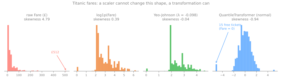
Box-Cox
\(x' = (x^\lambda - 1)/\lambda\), \(\lambda = 0\) means \(\log x\); \(\lambda\) by maximum likelihood. Needs \(x > 0\): refuses the free tickets.
Yeo-Johnson
accepts zero and negatives. \(\lambda = -0.098\), close to a log → skewness −0.04.
QuantileTransformer
replaces each value by its rank → −0.94; the 15 free tickets pile up at −5.20.
Encoding: three kinds of categories
nominal
no order: port, color, city
→ one-hot
ordinal
a real order: ticket class, education, size S < M < L
→ integers in that order
binary
two categories: Sex
→ one 0/1 column
OrdinalEncoder numbers the ports alphabetically: Cherbourg = 0, Queenstown = 1, Southampton = 2. What does a distance now believe about them?Integer codes invent distances
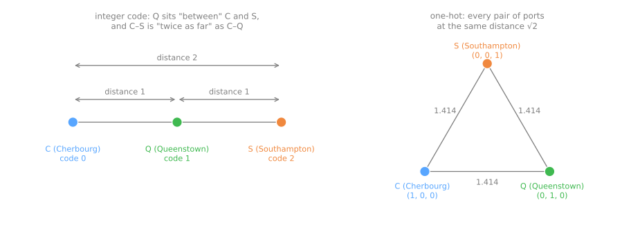
Codes: Q sits "between" C and S, and C–S is "twice as far" as C–Q. One-hot: every pair at \(\sqrt{1^2+1^2} = 1.414\).
Survival by port: C 0.554, Q 0.390, S 0.337. Steps of 16.4 and 5.3 points: one slope on the codes cannot represent both.
Ordinal: you declare the order
OrdinalEncoder().fit(levels).categories_
# ['bachelor', 'high school', 'master']   alphabetical!
OrdinalEncoder(categories=[['high school', 'bachelor', 'master']])
# codes now follow the real order: 0, 1, 2
The alphabet puts high school between bachelor and master.
Pclass is already 1, 2, 3. Ordinal (one column) or nominal (three one-hot columns) is a modeling choice: ordinal assumes 1st → 2nd matters as much as 2nd → 3rd.One-hot: two practical options
unseen categories
Trained on S, C, Q; a passenger from Belfast (B) arrives.
Default: ValueError, the prediction crashes.
handle_unknown='ignore': B becomes 0 0 0, "none of the categories I know".
drop='first'
C + Q + S = 1 on every row: the intercept's column. Rank 3 for 4 columns, so the weights are not unique.
Dropping C (the reference) restores full rank.
drop='first' for linear models with an intercept and no penalty. Keep every column for trees, k-NN and regularized models.High cardinality, and target encoding
Ticket has 681 distinct values for 891 rows: one-hot would create 681 columns of almost only zeros, a recipe for overfitting.
- First look for the structure inside: the deck letter of
Cabin, the title inName(Mr, Miss, Mrs, Master...). - Then group rare levels:
min_frequency=10keeps 4 titles and merges the other 13. - Target encoding: replace each category by the mean of the target in it. One column, whatever the cardinality.
Target encoding leaks
| encoding of pure noise | train | test |
|---|---|---|
| naive per-category mean | 0.775 | 0.505 |
TargetEncoder (cross-fitted) | 0.496 | 0.505 |
- Most tickets appear once or twice, so a row's encoded value is mostly its own label: the model learns to read the answer, not to predict it.
- Cross-fitting:
fit_transformencodes each fold with means from the other folds, so no row sees its own label; rare categories are shrunk toward the global mean.
fit_transform on train, transform on test. Target-free options: frequency encoding, hashing.Missing values: why is it missing?
| mechanism | what it means | Titanic example |
|---|---|---|
| MCAR, missing completely at random | depends on nothing | the 2 missing Embarked, plausibly |
| MAR, missing at random | depends on other observed columns | Age, missing more in 3rd class |
| MNAR, missing not at random | depends on the missing value itself | Cabin: no cabin of their own |
Age missing, by class
1st 13.9% · 2nd 6.0% · 3rd 27.7%
survival
age known 40.6% · age missing 29.4%
dropna() would cost 177 rows (19.9%), mostly 3rd class: the passengers who died most would be under-represented.Filling with one value shrinks the variance
Six values, two missing: 2, 4, ?, 6, ?, 8. Observed mean 5, variance \((9+1+1+9)/4 = 5\).
The imputed 5s add nothing to the squared deviations but add to the count: \(20/6 = 3.33\), the old variance times \(4/6\), the fraction observed.
Titanic ages
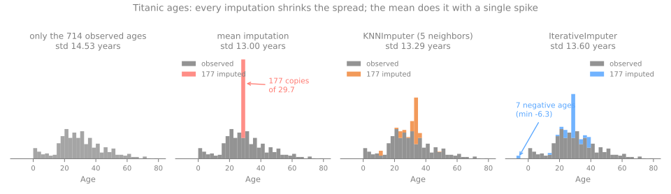
std 14.53 → 13.00, exactly the predicted \(\times\sqrt{713/890}\)
the cost
177 passengers share one invented age, 29.7
Imputing from the other columns
KNNImputer
average of the \(k\) most similar rows (needs comparable scales). Mr. James Moran, fare £8.46, no age: nearest fares £7.925 (26 y) and £7.25 (22 y) → 24. The mean says 30.25.
IterativeImputer
a regression of each column on the others, cycled (MICE). It produced 7 negative ages: it does not know that age is positive.
Keep the fact that it was missing
imp = SimpleImputer(strategy='median', add_indicator=True)
imp.get_feature_names_out()   # ['Age' 'missingindicator_Age']
# passenger 1: [22, 0]    passenger 6: [28, 1]
Missing age goes with lower survival (29.4% against 40.6%). The flag costs one column and lets the model decide whether missingness is informative. For categories: a category of its own, 'unknown'.
The preprocessing map
Per column: missing values → shape → scale, every step fitted on the training rows. Click the answers to build a recipe.
Which families care about which step
| model family | scaling | shape | encoding | missing values |
|---|---|---|---|---|
| k-NN, k-means, SVM, PCA | required | helps | one-hot | must be imputed |
| linear/logistic regression, neural networks | required | helps | one-hot, drop='first' if no penalty | must be imputed |
| trees, random forests, gradient boosting | not needed | not needed | ordinal codes are fine | scikit-learn's trees accept NaN |
Lab: preparing the Titanic for a model
- Inventory:
Survivedis the target,PassengerIdgoes out,Pclassis a category stored as a number. - Split first: 712 train, 179 test, stratified.
- Impute
Age(median), encodeSex,Embarked,Pclass(one-hot), scale the numbers. - All in one
ColumnTransformer: 12 columns, noNaN, no text.
Lab notebook (Jupyter or Colab, File → Upload notebook).
Same model, same data, different scaler
| numeric columns | test accuracy |
|---|---|
| baseline (always "did not survive") | 0.615 |
| k-NN, no scaling | 0.676 |
k-NN, StandardScaler | 0.821 |
k-NN, MinMaxScaler | 0.804 |
k-NN, RobustScaler | 0.771 |
Without scaling, neighbors are chosen almost only by fare (93.1% of the distance).
179 test passengers: each is worth 0.56 points, so the ranking between scalers is not reliable.
Summary
- Raw units decide distances by accident: scale what distances, variances and gradients use.
- Scalers differ in center and spread; outliers set the scale except for
RobustScaler. - A scaler cannot fix shape: log1p, Yeo-Johnson, then scale.
- One-hot for nominal, declared order for ordinal; target encoding only cross-fitted.
- Ask why it is missing; imputation shrinks spread; keep a flag.
- Fit on train, transform everything else.