Random Forest
The decision trees lesson ended on the decision tree's chronic defect: it is unstable. Refit it on a slightly different sample and the root question changes, the leaves change, and so do many predictions; the trees are about equally accurate, but each is wrong on different rows. The same lesson ended with a hint: letting many such trees vote beat every one of them. This lesson turns that hint into a method. Leo Breiman's idea (bagging, 1996; random forests, 2001) is not to fight the variance of one tree but to average many different trees and let their errors cancel. The result is one of the most reliable algorithms in machine learning: a strong default for tabular data that needs almost no tuning, estimates its own error for free, and trains in parallel.
The lesson first measures why averaging works and what limits it (the correlation between the members), then builds the forest in two steps, bootstrap samples and random feature subsets, and measures each one. Every number quoted comes from the code blocks or from the figure scripts next to this page.
How this lesson is organized
The lesson has two approaches. Each has slides, text and a lab to do in class on Colab; the quiz at the end covers the fundamental one. Start with the fundamental approach: the advanced one builds on it.
| Fundamental approach | Advanced approach | |
|---|---|---|
| question | Why does the average of many unstable trees beat every one of them, and how does a forest make them different? | Where averaging stops helping, which knobs matter, and how to read (and not read) a forest |
| content | the variance of an average, the bootstrap, bagging, the boundary smoothed by the vote, max_features and decorrelation, out-of-bag evaluation, how many trees | Condorcet's vote and correlation, the \(\rho\sigma^2\) floor measured, hyperparameters, feature importance and its biases, Extra-Trees, extrapolation, cost |
| in-class lab | spam filter: from one tree to a forest, steps 1 to 7 | tune, pick the threshold and test, steps 8 to 11 |
| by the end, you can | explain why the vote beats the trees; say what the bootstrap leaves out; use the OOB error instead of a validation split; know when to stop adding trees | tune max_features and min_samples_leaf; pick a threshold from OOB predictions; distrust impurity importance; know what a forest cannot do |
Both labs use the same notebook on Colab (in Portuguese): the fundamental part runs from step 1 to 7, the advanced part from step 8 to 11. Everything runs in the browser; there is nothing to download.
Fundamental approach
One question drives this part: how can an average of poor models be a good model? The answer has two conditions — reasonable members and weakly correlated errors — and the forest is built to meet both: the bootstrap gives every tree a different sample, and drawing the features at every split stops them from all starting with the same question. As a bonus, the rows each tree did not see give a validation for free.
This part follows one path in four stages, drawn below: 1. why averaging works; 2. bootstrap and bagging; 3. decorrelate the trees; 4. validate out-of-bag. Each stage links to its section, and in the slides a strip at the bottom shows which stage you are in.
- Why averaging worksthe variance of an average and its floor ρσ²
- Bootstrap and baggingresample, grow deep trees, vote
- Decorrelate the treesdraw
max_featurescandidates at every split - Validate out-of-bagthe out-of-bag (OOB) error; how many trees
Fundamental approach slides
Click the slides and use the ← → arrows to navigate; F opens full screen and Esc shows every slide. Open the slides in a new tab
1. Why averaging works
Stage 1. In 1907 Francis Galton looked at the 787 tickets of a weight-guessing contest at an English livestock fair: visitors paid sixpence to guess the weight of an ox once slaughtered and dressed. The individual guesses were all over the place, but their median was 1,207 lb; the ox weighed 1,198 lb (Galton, 1907). The crowd was better than almost every member of it, because the individual errors, pointing in different directions, canceled.
The arithmetic behind it is short. Take \(n\) estimates \(X_1, \dots, X_n\), each with variance \(\sigma^2\), and average them. If every pair has correlation \(\rho\), then
Two terms. The second one shrinks as \(n\) grows. The first one, \(\rho\sigma^2\), does not depend on \(n\) at all: it is the part of the error that all the estimators share, and no amount of averaging removes it. A simulation confirms the formula. Each estimator is a shared error plus its own error, mixed so that the variance is 1 and the correlation is \(\rho\):
import numpy as np

rng = np.random.default_rng(0)
reps = 20_000                                    # repeat the experiment 20,000 times
print(" rho    n   variance of the mean   formula")
for rho in [0.0, 0.3]:
    for n in [1, 10, 100]:
        shared = rng.normal(size=(reps, 1))      # the error all n estimators share
        own = rng.normal(size=(reps, n))         # each estimator's own error
        est = np.sqrt(rho) * shared + np.sqrt(1 - rho) * own   # variance 1, pairwise correlation rho
        print(f"{rho:4.1f} {n:4d}   {est.mean(axis=1).var():20.3f}   {rho + (1 - rho) / n:7.3f}")
 rho    n   variance of the mean   formula
 0.0    1                  1.015     1.000
 0.0   10                  0.100     0.100
 0.0  100                  0.010     0.010
 0.3    1                  0.998     1.000
 0.3   10                  0.374     0.370
 0.3  100                  0.312     0.307
With independent estimators (\(\rho = 0\)), averaging 10 divides the variance by 10 and averaging 100 divides it by 100. With \(\rho = 0.3\), 10 estimators bring the variance from 1 to 0.37, and 100 estimators only to 0.31: ten times more work for almost nothing, because the floor is \(\rho\sigma^2 = 0.3\). The left panel of the figure draws the formula for four correlations, with the simulation as dots (figure script):
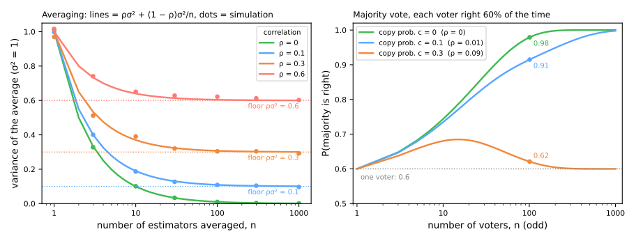
That is the entire design brief of a random forest: members that are individually good (small \(\sigma^2\)) and as little correlated as possible (small \(\rho\)).
2. The bootstrap: new training sets from the one you have
Stage 2. To average many trees we need many training sets, and we only have one. The bootstrap (Efron, 1979) manufactures new ones: draw \(n\) rows with replacement from the \(n\) rows you have. By hand, with 10 rows:
rng = np.random.default_rng(0)
rows = np.arange(10)                             # a training set of 10 rows, numbered 0..9
boot = rng.choice(rows, size=10, replace=True)   # a bootstrap sample: 10 draws with replacement
counts = np.bincount(boot, minlength=10)
print("drawn:      ", np.sort(boot))
print("times drawn:", counts)
print("left out:   ", rows[counts == 0])
The sample has 10 rows, like the original, but row 0 appears three times, row 8 twice, and rows 4, 7 and 9 not at all. A tree grown on it sees a slightly distorted version of the data, with some rows weighted up and some missing, and that is exactly the kind of perturbation that makes an unstable tree change.
How many rows are left out? One draw misses a given row with probability \(1 - 1/n\); \(n\) independent draws all miss it with probability \((1 - 1/n)^n\), which tends to \(1/e\):
print("    n   (1 - 1/n)^n   simulated")
for n in [10, 100, 1000]:
    left_out = [np.mean(np.bincount(rng.integers(0, n, n), minlength=n) == 0) for _ in range(10_000)]
    print(f"{n:5d}   {(1 - 1 / n)**n:11.4f}   {np.mean(left_out):9.4f}")
print(f"limit 1/e = {np.exp(-1):.4f}")
Already at \(n = 100\), a bootstrap sample leaves out 36.6% of the rows and contains the other 63.4%, some of them several times. The left-out rows will be useful later: for the tree that did not see them, they are fresh data.
The table below shows six bootstrap samples of the same 10 rows, one per column: each cell says how many times the row was drawn for that tree; the gray ones are rows left out (figure script):
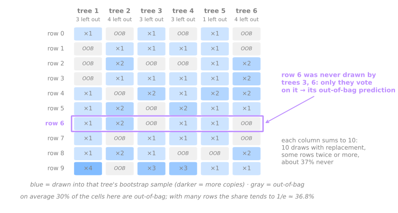
Every column adds up to 10 draws; some rows go in two, three or four times and others not at all. Keep the gray cells in mind: in section 5 they become a validation for free.
3. Bagging
Bagging (bootstrap aggregating, Breiman, 1996) is the combination of the two ideas: grow \(B\) trees, each on its own bootstrap sample, usually to full depth, and average their predictions (regression) or let them vote (classification).
Variance, measured
The claim is that bagging reduces variance and leaves bias alone. That can be measured directly, because variance is about different training sets. Draw 100 training sets of 100 points from the same process, \(y = \sin x + 0.5 \sin 3x\) plus noise with standard deviation 0.3, fit each model on every one of them, and watch the predictions at 100 fixed points. The bias² is how far the average prediction (over the 100 fits) is from the true function; the variance is how much the 100 predictions scatter around their own average. Their sum plus the noise variance, 0.09, is the expected squared error on a new point:
from sklearn.ensemble import BaggingRegressor
from sklearn.tree import DecisionTreeRegressor


def truth(x):
    return np.sin(x) + 0.5 * np.sin(3 * x)


x_grid = np.linspace(0.2, 6.1, 100).reshape(-1, 1)     # 100 fixed points where we watch the models
models = {'tree, max_depth=3': DecisionTreeRegressor(max_depth=3),
          'tree, full depth': DecisionTreeRegressor(),
          'bagging, 100 full trees': BaggingRegressor(DecisionTreeRegressor(), n_estimators=100,
                                                      random_state=0)}
preds = {name: [] for name in models}
members = []                                           # 10 of the bagged trees, for the next block
for s in range(100):                                   # 100 training sets from the same process
    r = np.random.default_rng(s)
    x = r.uniform(0, 2 * np.pi, (100, 1))
    y = truth(x[:, 0]) + r.normal(0, 0.3, 100)         # noise variance 0.09
    for name, model in models.items():
        preds[name].append(model.fit(x, y).predict(x_grid))
    members.append([t.predict(x_grid) for t in models['bagging, 100 full trees'].estimators_[:10]])

print(f"{'':24s} bias²   variance   expected test MSE")
for name, P in preds.items():
    P = np.array(P)                                    # 100 training sets × 100 points
    bias2 = ((P.mean(axis=0) - truth(x_grid[:, 0]))**2).mean()
    var = P.var(axis=0).mean()
    print(f"{name:24s} {bias2:.4f}  {var:.4f}     {bias2 + var + 0.09:.4f}")
                         bias²   variance   expected test MSE
tree, max_depth=3        0.0223  0.0274     0.1397
tree, full depth         0.0010  0.0883     0.1793
bagging, 100 full trees  0.0006  0.0413     0.1318
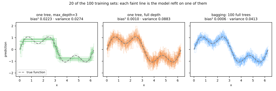
The three rows are the three ways out of the decision trees lesson's dilemma:
- The full tree has almost no bias (0.0010): on average it is right. But each fit chases the noise of its own training set, and the variance, 0.0883, is essentially the noise variance itself (0.09): a leaf with one point predicts that point's noise.
- Pruning to depth 3 cuts the variance to 0.0274, but pays with bias (0.0223): eight leaves cannot follow two superposed waves. That is the bias–variance trade-off of the model selection lesson, where every knob that lowers one raises the other.
- Bagging refuses the trade. It keeps the full trees' low bias (0.0006) and halves their variance (0.0413). Its expected error, 0.1318, is the lowest of the three.
Classification: the vote smooths the boundary
The same thing in two dimensions, on 300 noisy points of the "two moons" dataset, scored on 10,000 fresh points from the same process (figure script):
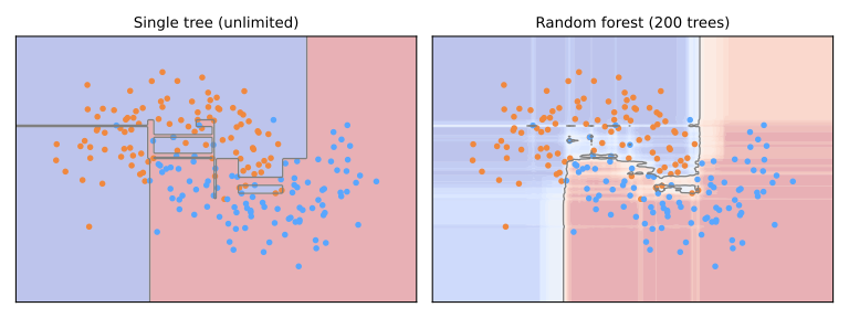
The middle panel is the point of the whole method. Each tree of the forest is worse than the single tree on the left (0.858 on average against 0.885), because it saw only about 63% of the distinct points and, at each split, only one of the two coordinates, drawn at random (the random forest's feature subsampling, explained below). The trees disagree wildly about where the boundary is, and each one draws its own islands. Yet their vote, on the right, scores 0.903, better than any of them: the islands are in different places for different trees, so they are outvoted, while the true shape, which every tree approximately finds, survives the vote. The color intensity is the fraction of trees voting for each class, a graded confidence that a single fully grown tree, with its pure leaves, cannot give.
What averaging does, and what it cannot do
The simulator below grows trees on bootstrap samples of 90 points, each split considering only one of the two coordinates, drawn at random. The left panel shows the individual trees; the right, their vote; the curve, the vote's error on new points (a test set from the same distribution) as trees are added:
Two things to notice, and the second is the one usually missed.
The left panel never improves. Add fifty trees and each of them is exactly as jittery as the first. Bagging does not produce better trees; it produces a better average of the same unstable trees.
The error curve flattens. Past a few dozen trees, more trees buy nothing. That is not a convergence bug: averaging attacks variance and leaves bias untouched, and the part of the variance the trees share, \(\rho\sigma^2\), stays too. If the flat part of that curve is too high, adding trees is the one thing guaranteed not to help: you need different trees (the next section), better features, or a different model. It is also why n_estimators is a budget question rather than a tuning question: more is never worse, just slower.
4. Random forests: decorrelating the trees
Stage 3. Bagged trees are correlated for a simple reason: they all see the same strong features. If one feature is by far the best first split, nearly every bootstrap sample will pick it at the root, the trees will start alike, and their mistakes will coincide. Breiman's second ingredient (2001), building on the random-subspace idea of Ho (1995, 1998) and the randomized trees of Amit & Geman (1997): at every split, only a random subset of max_features features is eligible. The best of those is chosen. A strong feature that is not drawn at a node cannot be used there, and other features get their chance.
The figure shows the mechanism on five trees and eight features, where f3 is by far the best first question (figure script):
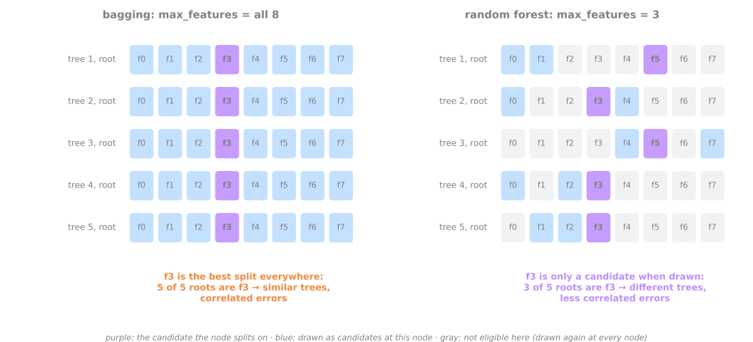
Each tree gets weaker, since it is often denied the best split. The trees also get less alike. The first section says which effect wins: the forest's variance is \(\rho\sigma^2 + (1-\rho)\sigma^2/B\), so lowering \(\rho\) can more than pay for a larger \(\sigma^2\). On the digits dataset (1,797 handwritten digits, 8×8 = 64 pixels each), with 5-fold cross-validation on a training split (the cross-validation lesson):
import pandas as pd
from sklearn.datasets import load_digits
from sklearn.ensemble import RandomForestClassifier
from sklearn.model_selection import StratifiedKFold, train_test_split

X, y = load_digits(return_X_y=True)                    # 1,797 images of 8×8 pixels, digits 0-9
X_train, X_test, y_train, y_test = train_test_split(X, y, test_size=0.25, stratify=y, random_state=0)
cv = StratifiedKFold(n_splits=5, shuffle=True, random_state=0)

rows = []
for m in [64, 20, 8, 3, 1]:                            # 64 = all pixels = plain bagging; 8 = sqrt(64)
    corr, tree_err, forest_err, roots = [], [], [], []
    for tr, va in cv.split(X_train, y_train):
        rf = RandomForestClassifier(n_estimators=200, max_features=m, random_state=0, n_jobs=-1)
        rf.fit(X_train[tr], y_train[tr])
        Xv, yv = X_train[va], y_train[va]
        wrong = np.array([rf.classes_[t.predict(Xv).astype(int)] != yv for t in rf.estimators_])
        C = np.corrcoef(wrong)                         # 200 × 200: do two trees fail on the same rows?
        corr.append(np.nanmean(C[np.triu_indices(200, 1)]))
        tree_err.append(wrong.mean())
        forest_err.append(1 - rf.score(Xv, yv))
        roots += [t.tree_.feature[0] for t in rf.estimators_]
    top_root = pd.Series(roots).value_counts().iloc[0] / len(roots)
    rows.append({'max_features': m, 'same root pixel': f"{top_root:.0%}",
                 'correlation': round(np.mean(corr), 3), 'one tree error': round(np.mean(tree_err), 3),
                 'forest error': round(np.mean(forest_err), 3)})
print(pd.DataFrame(rows).to_string(index=False))
 max_features same root pixel  correlation  one tree error  forest error
           64             66%        0.304           0.195         0.053
           20             24%        0.233           0.215         0.027
            8             10%        0.198           0.249         0.023
            3              6%        0.160           0.309         0.025
            1              4%        0.133           0.375         0.030
For each forest, wrong records which validation images each tree gets wrong, and correlation is the average correlation between two trees' mistakes: 1 would mean that they always fail on the same images, 0 that their failures are unrelated. Read the table from top to bottom:
- Plain bagging (all 64 pixels): 66% of the trees ask about the same pixel at the root. Their mistakes have correlation 0.304. Each tree errs on 19.5% of the images, and the forest on 5.3%.
max_features = 8(\(\sqrt{64}\), scikit-learn's default for classification): only 10% of the roots coincide, and the correlation drops to 0.198. Each tree is worse (24.9% error), but the forest is more than twice as good: 2.3% error.max_features = 1: each split takes a random pixel and only chooses its threshold. The correlation keeps falling (0.133), but the trees are now so weak (37.5% error) that the forest gets worse again (3.0%).
The figure runs the same experiment for twelve values of max_features (figure script):
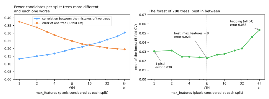
This is Breiman's strength–correlation trade-off: the forest wants trees that are strong and uncorrelated, and max_features trades one for the other. The optimum is usually broad and sits at a small fraction of the features; the defaults are \(\sqrt{d}\) for classification and, in scikit-learn, all features for regression (max_features=1.0, which makes RandomForestRegressor plain bagging unless you change it; Breiman suggested \(d/3\)).
A short history
Tin Kam Ho (1995, 1998) built "random decision forests" by growing each tree on a random subset of the features, the random subspace method. Amit & Geman (1997) randomized the features considered at each node, for recognizing shapes. Breiman had introduced bagging in 1996; his 2001 paper combined bootstrap samples with random feature selection at each split, named the result random forests, and gave the out-of-bag error estimate and the strength–correlation analysis used in this lesson. Geurts, Ernst & Wehenkel (2006) pushed the randomization further with Extra-Trees (below).
5. Out-of-bag evaluation: validation for free
Row by row
Stage 4. Every tree of a forest was grown on a bootstrap sample that left out about 37% of the rows. For that tree, those rows are out-of-bag (OOB): unseen data. So every training row has a set of trees that never saw it, and those trees can vote on it. Here is a forest of only 10 trees on the digits, and two training images:
small = RandomForestClassifier(n_estimators=10, random_state=0).fit(X_train, y_train)
for row in [15, 7]:
    print(f"row {row} (true digit {y_train[row]}):")
    for b, (tree, drawn) in enumerate(zip(small.estimators_, small.estimators_samples_)):
        times = (drawn == row).sum()                   # how often the bootstrap drew this row
        if times == 0:
            print(f"   tree {b}: out-of-bag, votes {int(tree.predict(X_train[[row]])[0])}")
row 15 (true digit 7):
   tree 0: out-of-bag, votes 4
   tree 2: out-of-bag, votes 7
   tree 3: out-of-bag, votes 7
   tree 7: out-of-bag, votes 4
   tree 8: out-of-bag, votes 7
   tree 9: out-of-bag, votes 7
row 7 (true digit 9):
   tree 0: out-of-bag, votes 9
   tree 2: out-of-bag, votes 3
   tree 6: out-of-bag, votes 3
   tree 8: out-of-bag, votes 3
Image 15 (a 7) was left out by 6 of the 10 trees; four of them vote 7 and two vote 4, so its OOB prediction is 7, right. Image 7 (a 9) was left out by 4 trees, three of which vote 3: its OOB prediction is wrong. Doing this for every training row and counting the mistakes gives the OOB error, and 1 minus it is oob_score_. (scikit-learn averages the OOB trees' predicted probabilities rather than counting votes; with fully grown trees, whose leaves are almost always pure, the two coincide.) No row was ever scored by a tree that trained on it, so the estimate is honest, and it costs no extra fit.
OOB against cross-validation and the test set
from sklearn.model_selection import cross_val_score

rf = RandomForestClassifier(n_estimators=500, oob_score=True, random_state=0, n_jobs=-1)
rf.fit(X_train, y_train)
cv_acc = cross_val_score(RandomForestClassifier(n_estimators=500, random_state=0, n_jobs=-1),
                         X_train, y_train, cv=cv)
print(f"OOB accuracy        {rf.oob_score_:.3f}   (1 fit)")
print(f"5-fold CV accuracy  {cv_acc.mean():.3f} ± {cv_acc.std():.3f}   (5 fits)")
print(f"test accuracy       {rf.score(X_test, y_test):.3f}   (450 untouched images)")
OOB accuracy        0.975   (1 fit)
5-fold CV accuracy  0.977 ± 0.007   (5 fits)
test accuracy       0.976   (450 untouched images)
Three estimates of the same thing, and they agree within 0.002: the OOB estimate is as good as 5-fold CV here, at a fifth of the cost. Each OOB prediction comes from a sub-forest of about 37% of the trees, trained on about 63% of the distinct rows, so it is, if anything, slightly pessimistic, like a CV with small training folds. OOB is convenient for quick checks, for learning curves over n_estimators, and for choosing a decision threshold without a separate validation split (the lab does exactly that). It does not replace a proper cross-validation when you compare a forest with other models: they have no OOB estimate, and comparisons need the same folds for everyone (the cross-validation lesson).
How many trees?
Growing one forest tree by tree (warm_start=True) and recording the OOB error, the test error and, at a few sizes, the CV error (figure script):
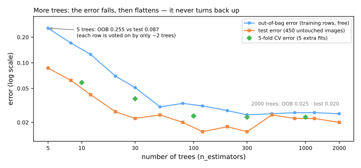
The error falls fast, then flattens, and it never turns back up: more trees cannot overfit, because each new tree only makes the average more stable (the \((1-\rho)\sigma^2/B\) term shrinks). The flat part wiggles by a few thousandths (one of the 450 test images is 0.0022) but shows no trend. The only price of more trees is time and memory. The left end also shows the one case where OOB misleads: with 5 trees, each row is out-of-bag for only about 2 of them, so its OOB "forest" is tiny, and the OOB error (0.255) is far worse than that of the actual 5-tree forest on the test set (0.087). Read the OOB error only once the forest has a few dozen trees.
Overfitting in a forest, when it happens, comes from the individual trees being too deep on noisy data, not from their number, and it is controlled with min_samples_leaf or max_depth.
6. Summary: the forest in five lines
- Averaging cuts variance, down to a floor. The variance of the mean of \(n\) members is \(\rho\sigma^2 + (1-\rho)\sigma^2/n\): the shared term, \(\rho\sigma^2\), does not fall with \(n\).
- The bootstrap gives each tree a different sample of the same rows; about 37% of them are left out of each tree.
- Bagging grows deep trees (low bias, high variance) on bootstrap samples and averages them: the bias stays, the variance falls.
max_featuresdraws the candidates of every split: individually worse trees, but less correlated ones — and a better forest.- The out-of-bag rows evaluate the forest without a validation split; more trees never make the error worse, they only cost time.
| symptom | what is happening | what to do |
|---|---|---|
| the OOB error curve went flat | averaging already removed the variance it can | stop adding trees |
| flat, but too high | the trees' bias or their correlation | deeper trees, another max_features, better features |
| OOB error much worse than the test error | too few trees: each row gets few OOB votes | only read the OOB error with a few dozen trees |
| forest barely better than bagging | one strong feature dominates every root | lower max_features |
Fundamental lab — a spam filter with forests
The problem. The Spambase dataset (Hopkins et al., 1999) was collected at Hewlett-Packard Labs: 4,601 e-mails, each described by 57 numbers, the frequency of 48 words and 6 characters (free, remove, $, !, ...) and three measures of runs of capital letters. The task: flag spam. You met it in the decision trees lesson, where fifty trees grown on bootstrap resamples voted better than any of them. Here we build the forest properly and ask what a spam filter must care about: a legitimate e-mail sent to the spam folder is worse than a spam that gets through, so precision on the spam class matters more than recall.
The workflow is the one from the validation lesson: lock a test set away, compare models on the same cross-validation folds, and touch the test set exactly once, at step 10. This part goes from a single tree to a forest and measures what the forest gains; tuning, the threshold and the test are left to the advanced lab.
How to do this lab in class (about 40 min, in pairs)
- Open the lab notebook on Colab (in Portuguese). There is nothing to download or install: Colab runs in the browser. To keep your answers, save a copy to your Drive (File → Save a copy in Drive) before editing. Run the cells in order, in a single session.
- This lab is steps 1 to 7 of the notebook. The advanced lab continues in the same notebook, from step 8.
- Every step starts with a Predict: answer it with your partner before running the cell. Getting the prediction wrong is what makes the result memorable.
- After running, compare with the output and the reading on this page. Every output here is exactly what the code prints.
- The Simulations ask you to write a small Python experiment: change one input and watch what happens to the output. No hand calculations. The solution is collapsed right below: try before opening it.
- Suggested pace: steps 1 to 3 in 10 min; steps 4 and 5 and the first simulation in 15 min; steps 6 and 7 and the second simulation in 15 min. Step 4 takes a few seconds to run.
Step 1 — load and look
Predict. Which words do you expect to see much more often in spam than in legitimate e-mail? Could some word signal "legitimate" just because of who collected the data?
import numpy as np
import pandas as pd
from sklearn.datasets import fetch_openml

pd.set_option('display.max_columns', 20)
pd.set_option('display.width', 120)
spam = fetch_openml(data_id=44, as_frame=True)       # Spambase (UCI): 4,601 e-mails
X = spam.data                                        # 57 numeric features
y = (spam.target == '1').astype(int)                 # 1 = spam, 0 = legitimate
print(X.shape)
print(y.value_counts())
tokens = ['word_freq_free', 'word_freq_remove', 'char_freq_%24', 'word_freq_george', 'word_freq_hp']
print(X[tokens].gt(0).groupby(y).mean().round(3))    # share of e-mails that contain each token
(4601, 57)
class
0    2788
1    1813
Name: count, dtype: int64
       word_freq_free  word_freq_remove  char_freq_%24  word_freq_george  word_freq_hp
class
0               0.090             0.015          0.104             0.277         0.373
1               0.546             0.421          0.612             0.004         0.028
4,601 e-mails: 1,813 spam (39.4%) and 2,788 legitimate. Every feature is a frequency (the percentage of the e-mail's words that are free, say) or a count, all non-negative and on very different scales; trees do not care, so there is no scaling anywhere in this lab. The table gives the share of e-mails that contain each token at least once, by class. free, remove and $ are classic spam markers: remove appears in 42.1% of the spam and 1.5% of the legitimate e-mails. The other two point the opposite way: george is in 27.7% of the legitimate e-mails and 0.4% of the spam, hp in 37.3% and 2.8%. That is not a law of spam. The legitimate e-mails came from the work and personal mailboxes of the people at HP Labs who built the dataset (George Forman among them), and its documentation notes that words like george indicate "not spam" only for that mailbox, which is useful for a personalized filter and nothing more. Keep it in mind for step 11. One caveat: 394 of these e-mails are exact duplicates of another one, which the decision-trees lesson drops as a duplicate-row leak. This lab keeps them, as most studies of this dataset do, so its cross-validated and test scores are slightly optimistic; rerunning it after X.drop_duplicates() is a good exercise.
Step 2 — lock the test set away
Predict. With 921 test e-mails, how many accuracy points is a single e-mail worth?
from sklearn.model_selection import train_test_split

X_train, X_test, y_train, y_test = train_test_split(
    X, y, test_size=0.2, stratify=y, random_state=42)
print(X_train.shape, X_test.shape)
print(f"spam share: train {y_train.mean():.3f} · test {y_test.mean():.3f}")
3,680 e-mails for development and 921 locked away until step 10, both with 39.4% spam thanks to stratify=y. On the test set, one e-mail is worth 0.11 points of accuracy.
Step 3 — a baseline and the folds everyone shares
Predict. If 39.4% of the e-mails are spam, how often is a model that calls everything legitimate right? And what is its ROC AUC?
from sklearn.dummy import DummyClassifier
from sklearn.model_selection import StratifiedKFold, cross_validate

cv = StratifiedKFold(n_splits=5, shuffle=True, random_state=42)
folds = {}                                           # the 5 fold scores of every model, for step 5


def evaluate(name, model):
    r = cross_validate(model, X_train, y_train, cv=cv, scoring=['accuracy', 'roc_auc'])
    folds[name] = r
    print(f"{name:14s} accuracy {r['test_accuracy'].mean():.3f} ± {r['test_accuracy'].std():.3f} · "
          f"ROC AUC {r['test_roc_auc'].mean():.3f} ± {r['test_roc_auc'].std():.3f}")


evaluate('dummy', DummyClassifier(strategy='most_frequent'))
Calling everything legitimate is right 60.6% of the time and ranks nothing (ROC AUC 0.5). Any accuracy must be read against 0.606. The cv object is created once and reused by every model and by the grid search, so all comparisons are made on the same five folds (the cross-validation lesson); folds keeps each model's five scores for the paired comparison of step 5.
Step 4 — one tree, bagging, random forest, Extra-Trees
Predict. Between one tree and the three ensembles, on which metric will the gap be larger, accuracy or ROC AUC? Why?
from sklearn.ensemble import ExtraTreesClassifier, RandomForestClassifier
from sklearn.tree import DecisionTreeClassifier

evaluate('one tree', DecisionTreeClassifier(random_state=0))
evaluate('bagging', RandomForestClassifier(n_estimators=200, max_features=None,   # all 57 features
                                           random_state=0, n_jobs=-1))
evaluate('random forest', RandomForestClassifier(n_estimators=200, random_state=0, n_jobs=-1))
evaluate('extra-trees', ExtraTreesClassifier(n_estimators=200, random_state=0, n_jobs=-1))
one tree       accuracy 0.916 ± 0.008 · ROC AUC 0.913 ± 0.007
bagging        accuracy 0.940 ± 0.006 · ROC AUC 0.978 ± 0.005
random forest  accuracy 0.953 ± 0.006 · ROC AUC 0.986 ± 0.004
extra-trees    accuracy 0.957 ± 0.007 · ROC AUC 0.987 ± 0.004
How to read it:
- One tree: 91.6% accuracy but a ROC AUC of only 0.913. A fully grown tree has pure leaves, so its "probabilities" are 0 or 1 and it cannot rank the e-mails it is unsure about; its AUC is little more than its balanced accuracy.
- Bagging:
RandomForestClassifier(max_features=None)is exactly bagging of trees, since every split may use all 57 features. Two hundred trees raise accuracy to 94.0% and, above all, ROC AUC to 0.978: the fraction of trees voting "spam" is a fine-grained score. - Random forest: letting each split consider only 7 random features (\(\sqrt{57}\), rounded down) adds another 1.3 points of accuracy (95.3%) and brings the AUC to 0.986. The decorrelation effect measured on the digits, again.
- Extra-Trees: 95.7% and 0.987, essentially the same as the forest.
The standard deviations (0.004–0.008) are small next to the gaps between the first three rows, but the fair comparison is fold by fold.
Simulation: is the forest better than its own trees? On the first fold of cv, fit a 200-tree forest and measure each tree's validation accuracy on its own: the mean, the best and the worst. Compare with the forest's vote and with a single tree grown on all the fold's rows. Does any tree of the forest reach the vote?
Solution
tr, va = next(cv.split(X_train, y_train))                       # the first fold
Xa, ya, Xv, yv = X_train.iloc[tr], y_train.iloc[tr], X_train.iloc[va], y_train.iloc[va]
forest = RandomForestClassifier(n_estimators=200, random_state=0, n_jobs=-1).fit(Xa, ya)
tree_acc = np.array([np.mean(t.predict(Xv.to_numpy()) == yv.to_numpy()) for t in forest.estimators_])
single = DecisionTreeClassifier(random_state=0).fit(Xa, ya).score(Xv, yv)
print(f"one tree on all the rows: {single:.3f}")
print(f"the forest's 200 trees:   mean {tree_acc.mean():.3f} · best {tree_acc.max():.3f} · worst {tree_acc.min():.3f}")
print(f"the forest's vote:        {forest.score(Xv, yv):.3f}")
one tree on all the rows: 0.928
the forest's 200 trees:   mean 0.900 · best 0.935 · worst 0.861
the forest's vote:        0.961
Each tree of the forest scores 0.900 on average, worse than the single tree grown on all the fold's rows (0.928): it saw only about 63% of the distinct e-mails and, at each split, only 7 of the 57 features. Not even the best of the 200 (0.935) comes close to the vote: 0.961. The forest beats all of its trees because they are wrong on different e-mails, and the vote cancels the errors that are not shared: the formula of section 1, with a larger \(\sigma^2\) and a much smaller \(\rho\).
Step 5 — paired differences, fold by fold
Predict. The forest is 1.3 accuracy points ahead of bagging, with fold standard deviations of about 0.006. Is that enough to declare a win? Which comparison settles the doubt?
for a, b in [('random forest', 'one tree'), ('random forest', 'bagging'), ('extra-trees', 'random forest')]:
    for metric in ['accuracy', 'roc_auc']:
        d = folds[a]['test_' + metric] - folds[b]['test_' + metric]
        print(f"{a} - {b:14s} {metric:8s} {d.round(3)}  ->  {d.mean():+.3f} ± {d.std():.3f}")
random forest - one tree       accuracy [0.033 0.034 0.052 0.031 0.035]  ->  +0.037 ± 0.007
random forest - one tree       roc_auc  [0.065 0.07  0.083 0.076 0.071]  ->  +0.073 ± 0.006
random forest - bagging        accuracy [0.018 0.01  0.011 0.007 0.02 ]  ->  +0.013 ± 0.005
random forest - bagging        roc_auc  [0.006 0.006 0.01  0.01  0.009]  ->  +0.008 ± 0.002
extra-trees - random forest  accuracy [ 0.001  0.005  0.005  0.015 -0.007]  ->  +0.004 ± 0.007
extra-trees - random forest  roc_auc  [ 0.001 -0.001  0.003  0.001  0.001]  ->  +0.001 ± 0.001
Each line subtracts two models' scores on the same fold:
- the forest beats the single tree in every fold, by 0.031 to 0.052 in accuracy (+0.037 ± 0.007) and by 0.065 to 0.083 in ROC AUC (+0.073 ± 0.006);
- the forest beats bagging in every fold too: +0.013 ± 0.005 in accuracy, +0.008 ± 0.002 in AUC. That is what the random choice of features is worth on this data;
- Extra-Trees against the forest: +0.004 ± 0.007 in accuracy, with one fold going the other way, and +0.001 ± 0.001 in AUC. The mean difference is no larger than its spread: by the rule of the cross-validation lesson, a tie.
With a tie, the choice is made on other grounds. We continue with the random forest, because it is trained on bootstrap samples and therefore has out-of-bag estimates, which the next steps use. (Extra-Trees skips the bootstrap by default.)
Step 6 — out-of-bag: the same estimate, one fit
Predict. Each tree leaves out about 37% of the e-mails. Will an estimate made only with the trees that did not see each e-mail land close to cross-validation, well above it, or well below it?
from sklearn.metrics import roc_auc_score

rf = RandomForestClassifier(n_estimators=200, oob_score=True, random_state=0, n_jobs=-1)
rf.fit(X_train, y_train)                             # one fit, on all of X_train
p_oob = rf.oob_decision_function_[:, 1]              # each e-mail scored only by trees that never saw it
print(f"OOB: accuracy {rf.oob_score_:.3f} · ROC AUC {roc_auc_score(y_train, p_oob):.3f}   (1 fit)")
print(f"CV:  accuracy {folds['random forest']['test_accuracy'].mean():.3f} · "
      f"ROC AUC {folds['random forest']['test_roc_auc'].mean():.3f}   (5 fits)")
in_bag = np.array([np.isin(np.arange(len(X_train)), s) for s in rf.estimators_samples_])
n_oob = (~in_bag).sum(axis=0)                        # trees that did NOT see each e-mail
print(f"out-of-bag trees per e-mail: mean {n_oob.mean():.1f} of 200 · min {n_oob.min()} · max {n_oob.max()}")
OOB: accuracy 0.953 · ROC AUC 0.986   (1 fit)
CV:  accuracy 0.953 · ROC AUC 0.986   (5 fits)
out-of-bag trees per e-mail: mean 73.6 of 200 · min 47 · max 100
The OOB estimate reproduces the 5-fold CV to the third decimal: accuracy 0.953 and ROC AUC 0.986 both ways, with one fit instead of five. The last line shows why it works: each e-mail was left out by 73.6 of the 200 trees on average (36.8%, the \(1/e\) of the bootstrap section), and never by fewer than 47. Those trees form a sizeable forest that never saw the e-mail.
oob_decision_function_ holds, for every training e-mail, the probability of spam computed only by those trees. That is an honest out-of-sample score for every training row, which step 9 uses to choose a threshold.
Step 7 — how many trees?
Predict. After a few dozen trees, does the OOB error keep falling, level off, or go back up?
import matplotlib.pyplot as plt

growing = RandomForestClassifier(warm_start=True, oob_score=True, random_state=0, n_jobs=-1)
sizes, oob_error = [10, 25, 50, 100, 200, 400], []
for B in sizes:
    growing.set_params(n_estimators=B).fit(X_train, y_train)   # warm_start: only the new trees are grown
    oob_error.append(1 - growing.oob_score_)
print(pd.Series(oob_error, index=pd.Index(sizes, name='trees'), name='OOB error').round(4).to_string())
plt.plot(sizes, oob_error, 'o-')
plt.xscale('log'); plt.xlabel('number of trees'); plt.ylabel('OOB error')
plt.show()
The OOB error falls from 7.55% with 10 trees to 4.62% with 100 and then stays flat: 4.67% with 200, 4.57% with 400. One e-mail is 0.027 points of OOB error, so the last three values differ by 2 to 4 e-mails: noise, not a trend. Two hundred trees are enough to compare configurations; the final model in step 9 uses 500, which costs only time.
Simulation: shallow trees, however many. Step 7 showed the OOB error leveling off with fully grown trees. Repeat with depth-3 trees (max_depth=3), for 10, 50, 200 and 400 trees. Does adding trees bring the shallow forest down to the error of the fully grown one?
Solution
print('trees   full trees   depth 3')
for B in [10, 50, 200, 400]:
    errs = []
    for depth in [None, 3]:
        f = RandomForestClassifier(n_estimators=B, max_depth=depth, oob_score=True, random_state=0, n_jobs=-1)
        errs.append(1 - f.fit(X_train, y_train).oob_score_)
    print(f"{B:5d}   {errs[0]:10.4f}   {errs[1]:7.4f}")
Both curves level off, but in different places: the forest of full trees near 4.6% OOB error, the forest of shallow trees near 8.7–8.9%, almost twice as much. From 200 to 400 trees the shallow forest does not even improve (0.0867 → 0.0886, a difference of seven e-mails: noise). Averaging removes variance; the error of a depth-3 tree is mostly bias — eight leaves are not enough to separate spam from legitimate mail — and 400 copies of a biased model are still biased. That is why forests use deep trees.
To close the fundamental part. In one sentence each: (1) why does a vote of 200 trees beat the best of them? (2) Why is the OOB error honest, if every tree was trained on X_train? (3) In which situation does adding trees not help at all?
Your turn (fundamental)
At home:
- Without the duplicates. Redo steps 3 to 6 after
X = X.drop_duplicates()(and the matchingy). How much do the CV accuracy and ROC AUC drop? Does the OOB error follow? - Smaller bootstrap samples. Use
max_samples=0.2(each tree sees 20% of the rows) and then0.5; compare CV ROC AUC and fit time with the default. How many out-of-bag trees does each e-mail get now? Does the OOB estimate still track CV? - A preview of the gradient boosting lesson. Add
evaluate('boosting', HistGradientBoostingClassifier(random_state=0))(fromsklearn.ensemble) to step 4 and compute its paired difference with the random forest in ROC AUC, as in step 5. Win, loss or tie?
Advanced approach
The fundamental part built the forest and showed why it works. This part shows where averaging stops helping and how to use a forest without fooling yourself: the majority vote under correlation, how much of bagging's error is the \(\rho\sigma^2\) floor, which hyperparameters really matter, why a forest's importances mislead, what Extra-Trees change, and what a forest cannot do. The code blocks continue those of sections 1 to 5.
This part follows one path in four stages, drawn below: 1. why the vote works; 2. tune what matters; 3. read the importances; 4. variants and limits. Each stage links to its section, and in the slides a strip at the bottom shows which stage you are in.
- Why the vote worksCondorcet's jury; the floor ρσ², measured
- Tune what matters
max_features,min_samples_leaf, enough trees - Read the importancesimpurity bias, permutation, shared credit
- Variants and limitsExtra-Trees, no extrapolation, cost
Advanced approach slides
Click the slides and use the ← → arrows to navigate; F opens full screen and Esc shows every slide. Open the slides in a new tab
7. Majority vote: Condorcet's jury theorem
Stage 1. Classifiers vote instead of averaging numbers, and the same logic applies. In 1785 the Marquis de Condorcet asked how often a jury decides correctly when each juror, independently, is right with probability \(p > 0.5\). With three jurors and \(p = 0.6\), the majority is right when all three are right or exactly two are:
The factor 3 counts which of the three jurors is the one who errs. For \(n\) jurors, the probability is a sum of binomial terms, one for each winning majority:
from math import comb


def majority_right(n, p):
    """P(more than half of n independent voters are right), each right with probability p."""
    return sum(comb(n, k) * p**k * (1 - p)**(n - k) for k in range(n // 2 + 1, n + 1))


for n in [1, 3, 11, 101, 1001]:
    print(f"n = {n:4d}: majority right with probability {majority_right(n, 0.6):.4f}")
n =    1: majority right with probability 0.6000
n =    3: majority right with probability 0.6480
n =   11: majority right with probability 0.7535
n =  101: majority right with probability 0.9791
n = 1001: majority right with probability 1.0000
Voters that are right only 60% of the time become, together, almost infallible: 0.7535 with 11 of them, 0.9791 with 101. The word that carries the whole theorem is independently. Suppose each voter, with probability \(c\), copies one shared opinion (a newspaper everyone reads, a feature every tree splits on first) and otherwise makes up its own mind:
def committee(n, p, c, reps=20_000, seed=0):
    """Each voter copies one shared opinion with probability c, otherwise votes on its own."""
    r = np.random.default_rng(seed)
    shared = r.random(reps) < p                  # is the shared opinion right?
    copies = r.random((reps, n)) < c             # which voters copy it
    own = r.random((reps, n)) < p                # the independent opinions
    right = np.where(copies, shared[:, None], own)
    return right, (right.sum(axis=1) > n / 2).mean()


for c in [0.0, 0.1, 0.3]:
    right, _ = committee(2, 0.6, c, reps=200_000)
    corr = np.corrcoef(right[:, 0], right[:, 1])[0, 1]
    acc = [committee(n, 0.6, c)[1] for n in [1, 11, 101, 1001]]
    print(f"c = {c:.1f} · correlation of two voters {corr:.2f} · majority right, n = 1/11/101/1001: "
          + '  '.join(f"{a:.3f}" for a in acc))
c = 0.0 · correlation of two voters -0.00 · majority right, n = 1/11/101/1001: 0.601  0.755  0.980  1.000
c = 0.1 · correlation of two voters 0.01 · majority right, n = 1/11/101/1001: 0.601  0.743  0.917  0.998
c = 0.3 · correlation of two voters 0.09 · majority right, n = 1/11/101/1001: 0.601  0.678  0.618  0.597
Every voter is still right 60% of the time on their own. But with \(c = 0.3\) the correlation between two voters is only 0.09 (\(c^2\), since both must copy), and it is enough to destroy the effect: a committee of 1,001 is right 59.7% of the time, no better than one voter. About 300 of the 1,001 voters copy the shared opinion and the other 700 split 60/40, so the copied block decides every vote, right or wrong. The right panel of the figure in section 1 shows the three curves. A little correlation (\(c = 0.1\)) slows the gain; more kills it.
8. Why bagging only halved the variance
The table of section 3 showed bagging 100 full trees taking the variance from 0.0883 (one full tree) down to 0.0413.
Why only halved, when 100 trees were averaged? The formula of the first section answers it. The trees are not independent: they were all grown from the same 100 points, noise included. Each bootstrap sample contains about 63% of those points, so two samples have about \(0.63^2 \approx 40\%\) of the points in common. Measure \(\sigma^2\) and \(\rho\) for the bagged trees, over the 100 training sets:
M = np.array(members)                                  # 100 training sets × 10 trees × 100 points
sigma2 = M.var(axis=0).mean()                          # variance of ONE bagged tree
Z = (M - M.mean(axis=0)) / M.std(axis=0)               # standardize over the training sets
rho = np.mean([(Z[:, i] * Z[:, k]).mean() for i in range(10) for k in range(i + 1, 10)])
print(f"one bagged tree: variance {sigma2:.4f} · correlation between two of them {rho:.2f}")
print(f"formula rho·σ² + (1 - rho)·σ²/100 = {rho * sigma2 + (1 - rho) * sigma2 / 100:.4f}")
one bagged tree: variance 0.0937 · correlation between two of them 0.44
formula rho·σ² + (1 - rho)·σ²/100 = 0.0417
One bagged tree has variance 0.0937 (a little more than a full tree on all the data, since it sees only 63% of the distinct rows), and two bagged trees have correlation 0.44 at the same point. The formula predicts \(0.44 \times 0.0937 + 0.56 \times 0.0937/100 = 0.0417\) for the average of 100, and the measured variance of bagging was 0.0413. Almost all of the remaining variance is the floor \(\rho\sigma^2\): adding more trees would not help. To go lower, the trees must become less correlated, which is what the feature draw of section 4 does.
9. Hyperparameters that matter, and those that barely do
Stage 2. A random forest has many knobs, but they are not equally important. To see which ones are worth tuning, change one at a time from the defaults and measure the 5-fold CV accuracy on the digits:
base = dict(n_estimators=200, random_state=0, n_jobs=-1)
study = {'n_estimators': [10, 30, 100, 300],
         'max_features': [1, 'sqrt', 0.5, None],
         'min_samples_leaf': [1, 3, 10, 30],
         'max_depth': [3, 6, 10, None],
         'criterion': ['gini', 'entropy']}
for param, values in study.items():
    scores = [cross_val_score(RandomForestClassifier(**{**base, param: v}), X_train, y_train, cv=cv).mean()
              for v in values]
    print(f"{param:16s}" + '  '.join(f"{str(v):>5s}: {s:.3f}" for v, s in zip(values, scores))
          + f"   range {max(scores) - min(scores):.3f}")
n_estimators       10: 0.941     30: 0.962    100: 0.976    300: 0.977   range 0.036
max_features        1: 0.970   sqrt: 0.977    0.5: 0.967   None: 0.947   range 0.030
min_samples_leaf    1: 0.977      3: 0.972     10: 0.947     30: 0.915   range 0.062
max_depth           3: 0.888      6: 0.957     10: 0.977   None: 0.977   range 0.089
criterion        gini: 0.977  entropy: 0.979   range 0.002
The fold standard deviation of these scores is about 0.007 (measured in the OOB section), so differences below 0.01 are noise.
n_estimatorsmatters until the curve flattens (0.941 with 10 trees, 0.976 with 100) and not after (0.977 with 300). Pick "enough", check the OOB curve, and stop.max_featuresis the forest's own knob: the defaultsqrtis best (0.977);None(bagging) loses 3 points. On other data the optimum can move, so it is the first thing to tune.min_samples_leafandmax_depthcontrol the depth of each tree. The defaults (fully grown trees) are best here: forests want deep, low-bias trees and let the averaging remove the variance. Shallow trees (depth 3: 0.888; leaves of at least 30 images: 0.915) add bias that no amount of averaging removes. On very noisy data, a moderatemin_samples_leaf(5–20) can help and makes the model smaller.criterion(Gini or entropy) changes nothing measurable (range 0.002), as for a single tree.class_weight('balanced', or'balanced_subsample', which recomputes the weights on each bootstrap sample) is for imbalanced classes, likeclass_weightin the ROC and imbalanced data lesson; the digits are balanced, so it is not studied here.
In practice: start from the defaults with a few hundred trees, tune max_features and min_samples_leaf with a small grid search on your cv, and spend any remaining effort on features. The lab does exactly this. Larger searches (random search, successive halving, Bayesian optimization) are the subject of AutoML.
10. Feature importance
Stage 3. A forest of hundreds of trees can no longer be read as a flowchart, so the question "which features does it use?" has to be answered by a number per feature. scikit-learn offers two, and they can disagree sharply.
- Impurity-based importance (MDI, mean decrease in impurity,
feature_importances_): for each feature, add up the impurity decrease of every split that uses it, weighted by the share of rows reaching that split, average over the trees, and normalize to sum to 1. It is computed from the training data, as a by-product of fitting, so it is free. The decision trees lesson showed its bias on a single tree. - Permutation importance (
sklearn.inspection.permutation_importance): on held-out data, shuffle one column, which breaks its link with the target while keeping its distribution, and measure how much the score drops. Repeat a few times and average. It costs one prediction pass per column and repeat, and it works for any model. It is developed further in Explainability.
Many distinct values attract splits
Strobl et al. (2007) showed that MDI favors features with many possible split points. To measure it, take the German credit data (1,000 loans, 20 attributes, 30% bad risks) and add two columns of pure noise: a serial number with 1,000 distinct values and a coin flip with 2:
from sklearn.datasets import fetch_openml
from sklearn.inspection import permutation_importance

credit = fetch_openml(data_id=31, as_frame=True)       # German credit: 1,000 loans, 20 attributes
Xc = credit.data.copy()
for col in Xc.select_dtypes('category'):
    Xc[col] = Xc[col].cat.codes                        # categories -> integer codes (fine for trees)
yc = (credit.target == 'bad').astype(int)              # 1 = bad credit risk (30%)
rng = np.random.default_rng(0)
Xc['random_id'] = rng.permutation(len(Xc))             # a serial number: 1,000 distinct values, no signal
Xc['coin'] = rng.integers(0, 2, len(Xc))               # a coin flip: 2 values, no signal
Xc_tr, Xc_te, yc_tr, yc_te = train_test_split(Xc, yc, test_size=0.3, stratify=yc, random_state=0)

forest = RandomForestClassifier(n_estimators=300, random_state=0, n_jobs=-1).fit(Xc_tr, yc_tr)
perm = permutation_importance(forest, Xc_te, yc_te, scoring='roc_auc', n_repeats=10,
                              random_state=0, n_jobs=-1)
imp = pd.DataFrame({'distinct values': Xc.nunique(),
                    'MDI': forest.feature_importances_,
                    'permutation': perm.importances_mean,
                    '± std': perm.importances_std})
imp['MDI rank'] = imp['MDI'].rank(ascending=False).astype(int)
imp['perm rank'] = imp['permutation'].rank(ascending=False).astype(int)
print(imp.sort_values('MDI', ascending=False).head(6).round(3).to_string())
print(imp.loc[['coin']].round(3).to_string())
                 distinct values    MDI  permutation  ± std  MDI rank  perm rank
credit_amount                921  0.129        0.007  0.013         1          8
random_id                   1000  0.099        0.002  0.007         2         14
duration                      33  0.087        0.056  0.014         3          2
age                           53  0.087        0.013  0.010         4          4
checking_status                4  0.086        0.144  0.026         5          1
purpose                       10  0.060        0.003  0.006         6         10
      distinct values   MDI  permutation  ± std  MDI rank  perm rank
coin                2  0.02       -0.002  0.003        17         22
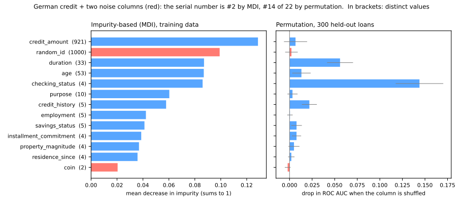
The serial number, noise by construction, is the second most important feature by MDI (0.099), ahead of the loan's duration, the applicant's age and the state of the checking account. Permutation importance on the 300 held-out loans puts it 14th of 22, with a drop in ROC AUC of 0.002 ± 0.007, smaller than its own standard deviation: shuffling it changes nothing, as it should. The coin flip, with only 2 values, is 17th by MDI and last (22nd) by permutation: few distinct values, few chances to fit noise.
The mechanism is the one from the decision trees lesson, multiplied by 300 trees. Deep in each tree, nodes hold a handful of rows, and a column with 1,000 distinct values offers hundreds of thresholds; one of them always separates those few rows a little better by chance, so the serial number gets chosen again and again, and every such split adds to its MDI. That impurity decrease is measured on the training rows, where the fitted noise really does "reduce impurity". The same bias inflates real features with many values: credit_amount (921 distinct values) is first by MDI but only 8th by permutation, while checking_status (4 values) is 5th by MDI and first by permutation, by far (figure script):
Correlated features share the credit
Permutation importance has a blind spot of its own. It asks "how much worse is the model if this one column is scrambled?", and if another column carries the same information, the answer is "not much". The cleanest test is an exact duplicate:
def importances(X_tr, X_te, cols):
    f = RandomForestClassifier(n_estimators=300, random_state=0, n_jobs=-1).fit(X_tr, yc_tr)
    p = permutation_importance(f, X_te, yc_te, scoring='roc_auc', n_repeats=10, random_state=0, n_jobs=-1)
    i = [list(X_tr.columns).index(c) for c in cols]
    return pd.DataFrame({'MDI': f.feature_importances_[i], 'permutation': p.importances_mean[i]}, index=cols)


print(importances(Xc_tr, Xc_te, ['checking_status']).round(3))
twin_tr = Xc_tr.assign(checking_copy=Xc_tr['checking_status'])   # an exact duplicate column
twin_te = Xc_te.assign(checking_copy=Xc_te['checking_status'])
print(importances(twin_tr, twin_te, ['checking_status', 'checking_copy']).round(3))
                   MDI  permutation
checking_status  0.086        0.144
                   MDI  permutation
checking_status  0.057        0.049
checking_copy    0.059        0.054
The information is the same, but with a twin in the table the two copies split the MDI (0.086 becomes 0.057 + 0.059) and each one's permutation importance falls to about a third (0.144 becomes 0.049 and 0.054). What makes the trees use both twins is max_features itself: at many nodes only one of the two is drawn as a candidate, so the forest learns to use either, and scrambling one leaves the other to do the work. Real data is full of near-twins (radius, perimeter and area of the same tumour; income and tax paid), and a feature that looks unimportant may simply have a substitute. Two practical rules follow:
- prefer permutation importance on held-out data to MDI, especially when features differ in their number of distinct values;
- before concluding that a feature does not matter, check its correlated partners: permute or drop the whole group together, or look at the model with tools that account for interactions, such as SHAP, in Explainability.
11. Extra-Trees and regression forests
Extra-Trees: random thresholds too
Stage 4. Extremely randomized trees (Geurts, Ernst & Wehenkel, 2006) go one step further: at each node, for each of the max_features candidate features, draw one random threshold instead of searching for the best one, and keep the best of these random splits. By default they also skip the bootstrap and grow every tree on all the rows. The trees are even less correlated, and each split is cheaper to find, since there is no threshold search. One import changes:
from sklearn.ensemble import ExtraTreesClassifier

for name, model in [('random forest', RandomForestClassifier(n_estimators=300, random_state=0, n_jobs=-1)),
                    ('extra-trees', ExtraTreesClassifier(n_estimators=300, random_state=0, n_jobs=-1))]:
    s = cross_val_score(model, X_train, y_train, cv=cv)
    nodes = np.mean([t.tree_.node_count for t in model.fit(X_train, y_train).estimators_])
    print(f"{name:14s} CV accuracy {s.mean():.3f} ± {s.std():.3f} · {nodes:.0f} nodes per tree")
random forest  CV accuracy 0.977 ± 0.010 · 329 nodes per tree
extra-trees    CV accuracy 0.981 ± 0.007 · 687 nodes per tree
On the digits, Extra-Trees are marginally ahead (0.981 against 0.977, well within one standard deviation). Their trees have twice as many nodes (687 against 329), since random thresholds split less efficiently, which costs memory and prediction time. It is a candidate worth one line in any comparison, as in the lab.
Regression forests, and what they cannot do
RandomForestRegressor averages regression trees exactly as the classifier averages votes. It inherits one limitation of its trees (the decision trees lesson): every prediction is an average of training targets, so it cannot predict outside the range of targets it has seen. Train on a straight line \(y = 3x\) for \(0 \le x \le 10\) and ask about larger \(x\):
from sklearn.ensemble import RandomForestRegressor
from sklearn.linear_model import LinearRegression

rng = np.random.default_rng(1)
x = np.linspace(0, 10, 100).reshape(-1, 1)              # training data only covers 0 <= x <= 10
y_line = 3 * x[:, 0] + rng.normal(0, 1, 100)           # a straight line, y = 3x, plus noise
x_new = np.array([[5], [10], [12], [20]])
print("x =            ", x_new[:, 0])
print("truth 3x:      ", 3 * x_new[:, 0])
print("random forest: ", RandomForestRegressor(random_state=0).fit(x, y_line).predict(x_new).round(1))
print("linear model:  ", LinearRegression().fit(x, y_line).predict(x_new).round(1))
x =             [ 5 10 12 20]
truth 3x:       [15 30 36 60]
random forest:  [15.6 29.6 29.6 29.6]
linear model:   [14.9 29.8 35.8 59.7]
Inside the training range, the forest is fine (15.6 for 15). Beyond it, it predicts 29.6 at \(x = 12\) and at \(x = 20\): the average of the last leaves, a flat line, however far you go. The linear model extrapolates the trend (59.7 for 60). For targets that grow over time (sales, prices), either model the trend separately or predict changes instead of levels.
12. Practical profile
A forest is the trees of the decision trees lesson, multiplied. That has a cost in size, which is easy to count:
import pickle
from sklearn.tree import DecisionTreeClassifier

models = {'one tree': DecisionTreeClassifier(random_state=0),
          'forest': RandomForestClassifier(n_estimators=300, random_state=0, n_jobs=-1),
          'forest, leaf 3': RandomForestClassifier(n_estimators=300, min_samples_leaf=3,
                                                   random_state=0, n_jobs=-1)}
for name, model in models.items():
    acc = cross_val_score(model, X_train, y_train, cv=cv).mean()
    model.fit(X_train, y_train)
    trees = getattr(model, 'estimators_', [model])        # a forest's trees, or the tree itself
    print(f"{name:14s} CV accuracy {acc:.3f} · {len(trees):3d} tree(s) · "
          f"{sum(t.tree_.node_count for t in trees):6d} nodes · "
          f"depth {np.mean([t.get_depth() for t in trees]):4.1f} · {len(pickle.dumps(model)) / 1e6:5.2f} MB")
one tree       CV accuracy 0.829 ·   1 tree(s) ·    293 nodes · depth 14.0 ·  0.04 MB
forest         CV accuracy 0.977 · 300 tree(s) ·  98696 nodes · depth 13.2 · 14.32 MB
forest, leaf 3 CV accuracy 0.971 · 300 tree(s) ·  65754 nodes · depth 11.7 ·  9.57 MB
On the digits, one tree scores 0.829 and the forest 0.977, but the forest stores over 300 times as many nodes: 14.32 MB once saved, for a training set of 1,347 small images, against 0.04 MB for the tree. Every prediction walks 300 root-to-leaf paths of depth about 13 instead of one. That is still fast, and the trees are independent, so it parallelizes across cores, but fully grown trees have roughly one leaf per handful of training rows, so the size grows with the data, which matters on a phone or behind a low-latency API. Larger leaves shrink it: min_samples_leaf=3 saves a third of the memory (9.57 MB) for 0.006 of accuracy.
| One decision tree | Random forest | Gradient boosting | |
|---|---|---|---|
| Trees | one, pruned | hundreds, deep, independent | hundreds, shallow, sequential |
| Attacks | — | variance (averaging) | bias (each tree fixes the previous errors) |
| Tuning needed | depth / pruning | little: max_features, leaf size | more: learning rate, number of trees, depth |
| Training | fast | parallel across trees | sequential (fast libraries exist) |
| Validation estimate | CV | OOB for free, or CV | CV / early stopping |
| Readable | yes, a flowchart | no; importances | no; importances |
| Extrapolates | no | no | no |
| Reach for it when | the model must be read or audited | a strong, robust baseline with little effort | the last points of accuracy on tabular data |
The forest's strengths: excellent accuracy with default settings; robust to outliers and to monotone transformations of the features, since splits only compare values; no scaling needed; captures interactions; OOB estimate; parallel training; hard to misuse. Its weaknesses: a large, slow-to-predict model compared with one tree or a linear model; no readable structure; no extrapolation; and on most tabular benchmarks a well-tuned gradient boosting model, the next lesson, edges it out.
Bagging vs boosting
Bagging builds trees independently, in parallel, and averages them to cut variance. Boosting, next lesson, builds them sequentially, each one correcting the errors of those before it, which attacks bias. Same building block, opposite strategies.
Advanced lab — tune, pick the threshold and test
The fundamental lab ended with a default 200-tree forest that scores 95.3% and whose OOB estimate reproduces cross-validation. This part tunes the two knobs that matter, uses the out-of-bag probabilities to pick a threshold that protects legitimate e-mail, opens the test set once, and asks where the forest looks. Continue in the same notebook, in the same session: the steps below use X_train, y_train, cv, folds and roc_auc_score from steps 1 to 7.
How to do this lab in class (about 30 min, in pairs)
- Continue in the Colab notebook, from step 8. If the session dropped, first run the cells of steps 1 to 7 (Runtime → Run before).
- As in the fundamental lab: Predict before running, compare with this page, and try the Simulations before opening the solution.
- Suggested pace: step 8 and the first simulation in 10 min (the grid takes a few seconds); steps 9 and 10 in 10 min; step 11 and the second simulation in 10 min.
Step 8 — tune max_features and min_samples_leaf
Predict. Fewer features per split make each tree weaker. Do you expect the best max_features near 1, near the default (7) or near 57? And leaves of 1 e-mail or of 5?
from sklearn.model_selection import GridSearchCV

grid = GridSearchCV(RandomForestClassifier(n_estimators=200, random_state=0, n_jobs=-1),
                    {'max_features': [1, 2, 4, 7, 15], 'min_samples_leaf': [1, 5]},
                    cv=cv, scoring='roc_auc')
grid.fit(X_train, y_train)
res = pd.DataFrame(grid.cv_results_)
print(res.pivot(index='param_min_samples_leaf', columns='param_max_features',
                values='mean_test_score').round(4))
best_std = res.loc[grid.best_index_, 'std_test_score']
print(f"best: {grid.best_params_} · ROC AUC {grid.best_score_:.4f} ± {best_std:.4f}")
ties = res[res['mean_test_score'] >= grid.best_score_ - best_std]
print(f"{len(ties)} of {len(res)} configurations within one std of the best:",
      list(zip(ties['param_max_features'], ties['param_min_samples_leaf'])))
param_max_features          1       2       4       7       15
param_min_samples_leaf
1                       0.9881  0.9875  0.9871  0.9857  0.9835
5                       0.9771  0.9804  0.9818  0.9823  0.9804
best: {'max_features': 1, 'min_samples_leaf': 1} · ROC AUC 0.9881 ± 0.0029
4 of 10 configurations within one std of the best: [(1, 1), (2, 1), (4, 1), (7, 1)]
Two patterns:
- Leaves of 1 beat leaves of 5 for every value of
max_featuresbut one: the forest wants deep trees, as on the digits. - Fewer features per split is better, slowly: from 0.9835 with 15 features to 0.9881 with 1. With
max_features=1, each split takes a feature at random and only chooses the threshold: on this data, maximal decorrelation pays.
The winner is max_features=1, min_samples_leaf=1, with ROC AUC 0.9881 ± 0.0029. But four of the ten configurations are within one standard deviation of it, including the default (max_features=7, 0.9857). Tuning bought 0.0024 of AUC, less than the fold-to-fold noise: forest defaults are hard to beat. We keep the grid's winner, which is also the fastest to train, since each split examines a single feature. Its 0.9881 is the best of ten scores measured on the folds that chose it, so it is slightly optimistic (the winner's curse of the cross-validation lesson).
Simulation: the search for free, with OOB. The grid of step 8 made 50 fits (10 configurations × 5 folds). Redo its min_samples_leaf=1 row with a single fit per configuration, reading the ROC AUC of the out-of-bag probabilities (oob_decision_function_). Does OOB rank the max_features values the way cross-validation does?
Solution
print('max_features   OOB ROC AUC   CV ROC AUC (grid)')
cv_auc = res[res['param_min_samples_leaf'] == 1].set_index('param_max_features')['mean_test_score']
for m in [1, 2, 4, 7, 15]:
    f = RandomForestClassifier(n_estimators=200, max_features=m, oob_score=True, random_state=0, n_jobs=-1)
    f.fit(X_train, y_train)                                    # one fit per configuration
    print(f"{m:12d}   {roc_auc_score(y_train, f.oob_decision_function_[:, 1]):11.4f}   {cv_auc[m]:.4f}")
max_features   OOB ROC AUC   CV ROC AUC (grid)
           1        0.9881   0.9881
           2        0.9886   0.9875
           4        0.9873   0.9871
           7        0.9855   0.9857
          15        0.9842   0.9835
With 5 fits instead of 25, OOB reproduces the cross-validation curve: both columns fall from 1 to 15 features and never differ by more than 0.0011. The order of the first two flips (OOB prefers 2, CV prefers 1), but each column separates them by 0.0005–0.0006, well within the winner's fold standard deviation (0.0029): the same tie seen from two sides. For a forest, OOB is a cheap way to sweep a knob; to compare with models of other families, which have no OOB, keep using the same cv.
Step 9 — a threshold that protects legitimate e-mail, chosen out-of-bag
Predict. To send at most 1% of legitimate e-mail to the spam folder, must the threshold go up or down from 0.5? Where can you choose it without touching the test set?
final = RandomForestClassifier(n_estimators=500, oob_score=True, random_state=0, n_jobs=-1,
                               **grid.best_params_).fit(X_train, y_train)
p_oob = final.oob_decision_function_[:, 1]
legit = (y_train == 0).to_numpy()
print(" threshold  legit flagged (of 2230)  spam caught")
for t in [0.5, 0.6, 0.65, 0.7, 0.8]:
    flag = p_oob >= t
    print(f"{t:10.2f}  {flag[legit].sum():5d} ({flag[legit].mean():.2%})        {flag[~legit].mean():.1%}")
thresholds = np.arange(0.50, 0.96, 0.05)
chosen = next(t for t in thresholds if (p_oob[legit] >= t).mean() <= 0.01)
print(f"chosen threshold: {chosen:.2f}")
 threshold  legit flagged (of 2230)  spam caught
      0.50     52 (2.33%)        93.2%
      0.60     31 (1.39%)        88.8%
      0.65     25 (1.12%)        86.1%
      0.70     19 (0.85%)        82.8%
      0.80      9 (0.40%)        73.5%
chosen threshold: 0.70
The policy comes from the problem, not from the data: at most 1% of legitimate e-mails may go to the spam folder. Choosing a threshold needs predictions on rows the model did not train on; in the ROC and imbalanced data lesson that cost a validation split. Here the out-of-bag probabilities provide them for all 3,680 training e-mails, at no cost.
At the default threshold of 0.5, the forest would flag 52 of the 2,230 legitimate training e-mails (2.33%), more than twice the budget. The first threshold on the grid that meets it is 0.70: 19 legitimate e-mails flagged (0.85%), while still catching 82.8% of the spam. The threshold is now fixed, before the test set is opened.
Step 10 — the one and only test
Predict. At the chosen threshold, will the share of legitimate e-mails lost on the test set land near the 0.85% that OOB predicted? And spam recall: up or down from the 0.5 threshold?
from sklearn.metrics import confusion_matrix, precision_score, recall_score

p_test = final.predict_proba(X_test)[:, 1]
print(f"test ROC AUC {roc_auc_score(y_test, p_test):.3f}")
for t in [0.5, chosen]:
    pred = (p_test >= t).astype(int)
    tp, fn, fp, tn = confusion_matrix(y_test, pred, labels=[1, 0]).ravel()
    print(f"threshold {t:.2f}: legit lost {fp} of {tn + fp} · spam missed {fn} of {fn + tp} · "
          f"precision {precision_score(y_test, pred):.3f} · recall {recall_score(y_test, pred):.3f}")
test ROC AUC 0.984
threshold 0.50: legit lost 14 of 558 · spam missed 32 of 363 · precision 0.959 · recall 0.912
threshold 0.70: legit lost 5 of 558 · spam missed 72 of 363 · precision 0.983 · recall 0.802
The ROC AUC on the 921 test e-mails is 0.984, close to the CV estimate of 0.988 (which, as the best of ten configurations, was slightly optimistic). Then the two thresholds, both fixed before this step:
- at 0.5, 14 of the 558 legitimate e-mails are sent to spam (2.5%): precision 0.959, recall 0.912;
- at 0.70, only 5 are (0.9%, where the OOB estimate had predicted 0.85%): precision 0.983. The price is recall: 72 of the 363 spam e-mails now reach the inbox, against 32.
Nine fewer lost e-mails cost forty more spams in the inbox. Whether that trade is right is a product decision; what the lab shows is that it can be made on out-of-bag predictions and then confirmed, once, on the test set. Reporting both rows is not choosing on the test: neither threshold was changed after seeing it.
Step 11 — what does the forest look at?
Predict. Will a column of serial numbers, with no signal at all, rank high in either of the two importances? Which one?
from sklearn.inspection import permutation_importance

rng = np.random.default_rng(0)
Xn_train = X_train.assign(random_id=rng.permutation(len(X_train)))   # plus one column of pure noise
Xn_test = X_test.assign(random_id=rng.permutation(len(X_test)))
probe = RandomForestClassifier(n_estimators=200, random_state=0, n_jobs=-1,
                               **grid.best_params_).fit(Xn_train, y_train)
perm = permutation_importance(probe, Xn_test, y_test, scoring='roc_auc', n_repeats=10,
                              random_state=0, n_jobs=-1)
imp = pd.DataFrame({'MDI': probe.feature_importances_, 'permutation': perm.importances_mean,
                    '± std': perm.importances_std}, index=Xn_train.columns)
imp['MDI rank'] = imp['MDI'].rank(ascending=False).astype(int)
imp['perm rank'] = imp['permutation'].rank(ascending=False).astype(int)
print(imp.sort_values('permutation', ascending=False).head(10).round(4))
print(imp.loc[['random_id']].round(4))
                     MDI  permutation   ± std  MDI rank  perm rank
char_freq_%21     0.0625       0.0046  0.0013         1          1
word_freq_free    0.0443       0.0039  0.0012         7          2
word_freq_hp      0.0273       0.0037  0.0008        11          3
word_freq_remove  0.0437       0.0033  0.0015         8          4
word_freq_edu     0.0177       0.0030  0.0006        21          5
word_freq_george  0.0162       0.0029  0.0008        25          6
word_freq_you     0.0350       0.0021  0.0006         9          7
word_freq_1999    0.0161       0.0019  0.0003        27          8
word_freq_hpl     0.0177       0.0014  0.0004        20          9
word_freq_re      0.0140       0.0014  0.0004        28         10
              MDI  permutation   ± std  MDI rank  perm rank
random_id  0.0219      -0.0002  0.0004        13         54
We refit the chosen configuration with one extra column of pure noise, a random serial number, and compare the two importances. Permutation importance is measured on the test set: it has already given its verdict in step 10, and explaining the model changes no decision about it.
How to read it:
- The serial number is 13th of 58 by MDI, ahead of 45 real features, and 54th by permutation, with a drop of −0.0002 ± 0.0004: nothing. It is the bias of the decision trees lesson's single tree (and of the German credit example above), now in a forest.
- The two rankings disagree on the real features too:
georgeis 25th by MDI and 6th by permutation,199927th and 8th. Trust the permutation column. - The drops are small (at most 0.0046 of AUC for
!) because the words substitute for one another: with one of them scrambled, the others still identify most spam. - Five of the top ten (
hp,edu,george,1999,hpl) are traces of where the legitimate e-mails came from: a research lab, its people, its correspondents. They help on this test set, which comes from the same mailboxes, and would mislead in anyone else's. Importance tells you what the model uses, not what is true about spam, and a list like this is the best way to catch a dataset artifact before it reaches production.
Simulation: the importance of a pair of twins. word_freq_857 and word_freq_415 almost always appear together in these e-mails. On the probe of step 11, measure the test ROC AUC drop when shuffling each one alone and both together (with the same row permutation), ten times each. Is the joint drop larger than the sum of the individual ones?
Solution
print(f"correlation: {X_train['word_freq_857'].corr(X_train['word_freq_415']):.3f}")
base_auc = roc_auc_score(y_test, probe.predict_proba(Xn_test)[:, 1])
r2 = np.random.default_rng(0)
drops = {}
for cols in [['word_freq_857'], ['word_freq_415'], ['word_freq_857', 'word_freq_415']]:
    d = []
    for _ in range(10):
        Xs = Xn_test.copy()
        order = r2.permutation(len(Xs))
        Xs[cols] = Xs[cols].to_numpy()[order]                  # the same permutation for both columns
        d.append(base_auc - roc_auc_score(y_test, probe.predict_proba(Xs)[:, 1]))
    drops[' + '.join(cols)] = np.mean(d)
for k, v in drops.items():
    print(f"shuffle {k:30s}: ROC AUC drop {v:.5f}")
correlation: 0.998
shuffle word_freq_857                 : ROC AUC drop 0.00021
shuffle word_freq_415                 : ROC AUC drop 0.00019
shuffle word_freq_857 + word_freq_415 : ROC AUC drop 0.00067
The two columns have a correlation of 0.998: they are almost the same information. Shuffled alone, each one is barely missed (0.00021 and 0.00019), because its twin covers for it. Shuffled together, the drop is 0.00067, about 1.7 times the sum of the individual drops (0.00040). Read one column at a time, permutation importance underestimates a group of correlated features; this is the exact-twin experiment of section 10, now on real data. The numbers are small because these two words carry little weight in the model; the disproportion is what matters.
To close the lesson. In one sentence each: (1) why is the winner of step 8's grid not convincingly better than the defaults? (2) Why can the out-of-bag probabilities choose the threshold without spending the test set? (3) Why are george and hp important in this model and useless in a filter for someone else?
Your turn (advanced)
At home, with more time:
- Class weights against thresholds. Add
'class_weight': [None, 'balanced_subsample']to the grid of step 8. Does the winner's ROC AUC change? Refit it with each option and compare the OOB threshold that step 9 chooses. Why can class weights and thresholds end up doing the same job (the ROC and imbalanced data lesson)? - Without the HP Labs traces. Drop the columns
word_freq_hp,word_freq_hpl,word_freq_george,word_freq_labs,word_freq_labandword_freq_650fromXand redo steps 8 to 10. How much does the test ROC AUC drop? Is that model worse, or just more honest? min_samples_leafby OOB. With the winner'smax_features, sweepmin_samples_leafover 1, 2, 5, 10 and 20 reading only the out-of-bag ROC AUC, as in the step-8 simulation. Where is the best value, and what happens to the model's size (sum(t.tree_.node_count for t in f.estimators_))?
References
- Galton, F. "Vox Populi." Nature 75 (1907): 450–451 — the ox-weighing contest. DOI
- Condorcet, Marquis de. Essai sur l'application de l'analyze à la probabilité des décisions rendues à la pluralité des voix. Paris: Imprimerie Royale (1785) — the jury theorem.
- Efron, B. "Bootstrap Methods: Another Look at the Jackknife." The Annals of Statistics 7, no. 1 (1979): 1–26. DOI
- Breiman, L. "Bagging Predictors." Machine Learning 24, no. 2 (1996): 123–140. DOI
- Ho, T. K. "Random Decision Forests." Proceedings of the 3rd International Conference on Document Analysis and Recognition (ICDAR) (1995): 278–282. DOI
- Amit, Y.; Geman, D. "Shape Quantization and Recognition with Randomized Trees." Neural Computation 9, no. 7 (1997): 1545–1588. DOI
- Ho, T. K. "The Random Subspace Method for Constructing Decision Forests." IEEE Transactions on Pattern Analysis and Machine Intelligence 20, no. 8 (1998): 832–844. DOI
- Breiman, L. "Random Forests." Machine Learning 45, no. 1 (2001): 5–32 — bootstrap plus random features, out-of-bag estimates, strength and correlation. DOI
- Geurts, P.; Ernst, D.; Wehenkel, L. "Extremely Randomized Trees." Machine Learning 63, no. 1 (2006): 3–42. DOI
- Strobl, C.; Boulesteix, A.-L.; Zeileis, A.; Hothorn, T. "Bias in Random Forest Variable Importance Measures: Illustrations, Sources and a Solution." BMC Bioinformatics 8 (2007): 25. DOI
- Hastie, T.; Tibshirani, R.; Friedman, J. The Elements of Statistical Learning, 2nd ed. Springer (2009), chapter 15 — the variance of an average of correlated trees. DOI
- Hopkins, M.; Reeber, E.; Forman, G.; Suermondt, J. "Spambase." UCI Machine Learning Repository (1999) — the lab's dataset (OpenML 44). DOI
Quiz
The quiz covers the fundamental approach.