Machine Learning · Insper

Imbalanced Data

Advanced approach

What each remedy actually changes when the class of interest is 2%

The path of this part

What goes wrong2% fraud: high accuracy, low recall; is it the model or the threshold?
Three remediesclass weights, a moved threshold, resampling and SMOTE (Synthetic Minority Over-sampling Technique)
Side by sidefive approaches on the same split, one curve
Two pitfallsresampling before the split; distorted probabilities

Each stage answers one question: what does a rare class break? → what can we change: the loss, the cut or the rows? → what did each remedy really change? → how can a remedy fool you?

Stage 1 · What does a rare class break?

What goes wrong

Simulated fraud screening: 20,000 transactions, about 2% fraudulent, stratified split.

	value
accuracy of the dummy that never flags	0.9805
accuracy of the model	0.9838
transactions flagged at 0.5	23 of 4,000 (78 real frauds)
recall	0.231
ROC AUC (area under the ROC curve)	0.930

98.38% accuracy says nothing: the dummy already has 98.05%. But the ranking is good — in 93% of the pairs, the fraud gets the higher score.

The diagnosis matters

The median transaction gets probability 0.003; 60 of the 78 frauds sit below 0.5.
That is honest: with a 2% base rate, even a suspicious transaction is usually more likely legitimate than not.

The model is not blind. The problem is the threshold and the metric, not necessarily the model.

Each remedy below acts on a different part — some move the operating point, others the ranking — and they are easy to confuse.

Stage 2 · What can we change: the loss, the cut or the rows?

Three places to intervene

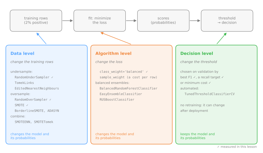
Data, algorithm and decision levels, each pointing at a stage of the path from training rows to decision, with the imblearn tools of each level

The first two levels change the model and its probabilities; the third only changes the decision. ✓ = measured in this lesson.

Remedy 1: class weights

\[ w_c = \frac{n}{k \cdot n_c} \qquad w_0 = \frac{12000}{2 \times 11767} = 0.510 \qquad w_1 = \frac{12000}{2 \times 233} = 25.751 \]

	AUC	AP	flagged	recall	precision
no weights	0.930	0.459	23	0.231	0.783
balanced	0.929	0.460	673	0.821	0.095

\(n\) rows, \(k = 2\) classes, \(n_c\) rows of class \(c\). AP = average precision, the summary of the precision–recall curve.

The ranking metrics barely move. What moves is the operating point at 0.5. The weights did not make the model better at separating frauds: they made it say "fraud" far more often.

What the weights did to the scores

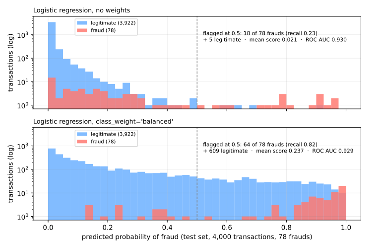
Histograms of predicted probability: without weights everything piles near 0; with weights all scores shift right

Same model, same separation: all the scores simply shifted to the right.

In logistic regression the slopes barely change and the intercept rises by 3.86 ≈ \(\log(n_0/n_1) = 3.92\): class_weight='balanced' is, in practice, a shifted threshold.

Remedy 2: move the threshold

If weights shift the intercept, you can shift the threshold directly and retrain nothing:

	flagged	recall	precision
no weights, \(t = 0.0194\) (training prevalence)	685	0.833	0.095
balanced, \(t = 0.5\)	673	0.821	0.095

Same operating point, without retraining: the two rules disagree on 42 of 4,000 transactions. This is often the cheapest remedy — and the only one you can change after deployment without touching the model.

Remedy 3: resampling

Undersampling: drops majority rows. Fast, throws information away (11,534 of 11,767).
Oversampling: duplicates the minority. Each fraud repeats ~50 times; flexible models memorize the copies.
SMOTE: creates new points between a minority point and one of its minority neighbors.

\[ x_{\text{new}} = x_i + \lambda\,(x_{nn} - x_i) \]

SMOTE on a 2-D toy set: synthetic points on segments between minority points

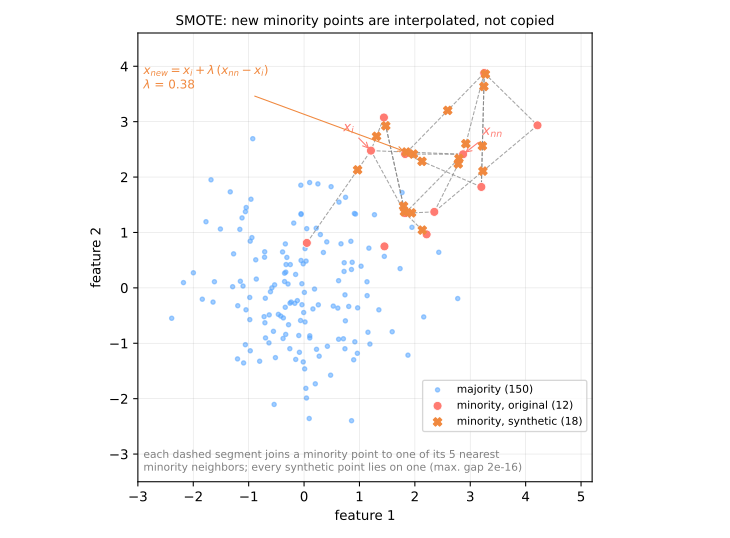
SMOTE only looks at minority neighbors: it will happily draw a segment across a region full of majority points. And resampling may only touch the training data — use the imblearn pipeline, which skips the sampler at predict.

Stage 3 · What did each remedy really change?

The five approaches, side by side

model	AUC	AP	R@0.5	F1@0.5	F1 tuned	\(t\)
no weights	0.930	0.459	0.231	0.356	0.449	0.22
balanced weights	0.929	0.460	0.821	0.170	0.439	0.91
undersampling	0.931	0.464	0.833	0.166	0.467	0.94
oversampling	0.929	0.461	0.821	0.169	0.437	0.91
SMOTE	0.929	0.453	0.821	0.176	0.462	0.94

Identical ranking across all five: AUC 0.929–0.931, AP 0.453–0.464. No remedy taught the model anything new about fraud.
R = recall; F1 = harmonic mean of precision and recall.
At the tuned threshold (the best F1 on validation) the differences vanish: F1 between 0.44 and 0.47. Same operating point, different numbers on the dial.

Resampling and weights mostly move the operating point; moving the threshold does the same, for free.

Five remedies, one curve

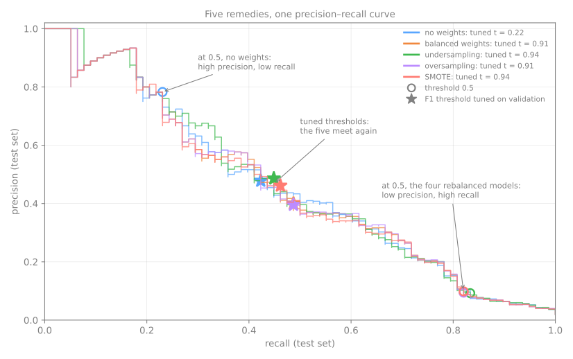
The precision–recall curves of the five remedies almost coincide; at 0.5 they sit at opposite ends of the curve; at the thresholds tuned on validation, the five meet again

Same ranking, same curve. The remedies change where 0.5 cuts; with a threshold tuned for each model, the five land on the same stretch.

Stage 4 · How can a remedy fool you?

Order matters: split, then resample

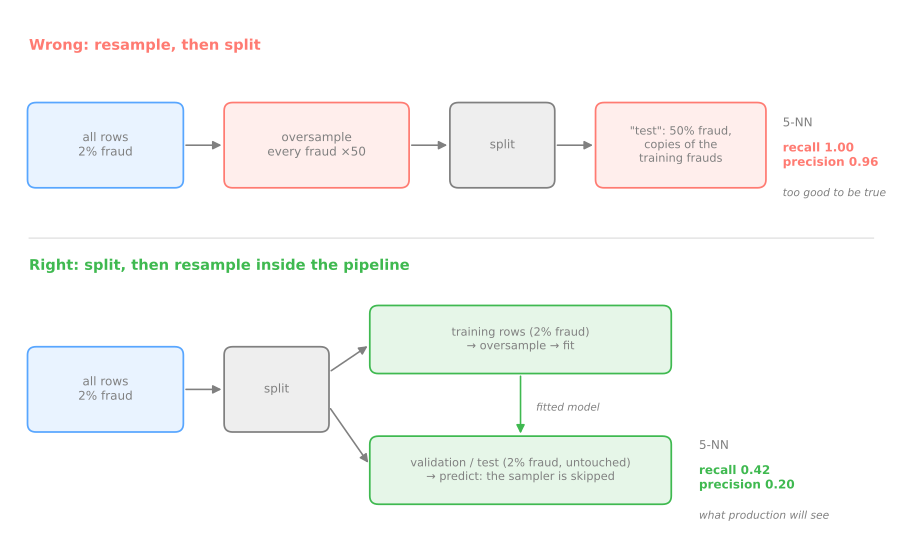
Wrong order: oversample everything and then split, giving a test set with 50% fraud and copies of the training rows; right order: split first and oversample only the training rows inside the pipeline

Pitfall 1: resampling before the split

sampler + model	wrong: R / P	right: R / P
oversampling + k-NN (5 neighbors)	1.00 / 0.96	0.42 / 0.20
oversampling + logistic	0.82 / 0.84	0.82 / 0.09
SMOTE + k-NN	1.00 / 0.92	0.56 / 0.12

the test set is contaminated: each fraud exists ~50 times, so almost every "test" fraud has identical copies in training; k-NN finds them;
the test set no longer has the real prevalence: 50% frauds instead of 2%, so a precision of 0.84 says nothing about production.

Pitfall 2: distorted probabilities

	mean probability
true fraud rate (test)	0.0195
no weights	0.0206
balanced weights	0.2370
SMOTE	0.2227
balanced, corrected	0.0208

Weights and resampling tell the model that frauds are 50% of the world, and it believes them. For a ranking or a yes/no decision at a tuned threshold, fine. If you need the number itself (an expected loss, a risk shown to a doctor, the \(t^*\) formula), not fine. For logistic regression the fix is exact: multiply the odds by \(n_1/n_0\).

A sensible order of attack

No resampling invents information the data does not have.

Advanced lab · about 35 min, in pairs

Remedies, threshold and the single test: steps 6 to 11

Same Colab notebook, from step 6 (Passo 6). New session? Runtime → Run before.
The goal was declared at the start of the fundamental lab: recall ≥ 0.80 on the malignant cases, with the best precision.
Simulations: the threshold that imitates the weights (step 6) and compare at a fair threshold (step 8).
Steps 9 to 11: choose model and threshold, the single test, and the coarse staircase of a k-NN.

Pace: steps 6 and 7 with the simulation in 15 min; step 8 and its simulation in 10 min; steps 9 to 11 in 10 min.