Support Vector Machines
The SVM (Cortes & Vapnik, 1995) crowned the statistical-learning era: a classifier derived from an elegant geometric principle — maximize the margin — with rigorous theory behind it and a trick that lets a linear method draw extremely non-linear boundaries. Before deep learning, SVMs were state of the art almost everywhere; they are still excellent on small-to-medium, high-dimensional problems.
You already know its two closest relatives. Like logistic regression, a linear SVM computes a score \(f(x) = w^\top x + b\) and predicts by its sign; its C is the same inverse regularization strength you tuned in cross-validation. Like k-NN, a kernel SVM predicts from the similarity of a new point to stored training points; what changes is that only a few of them (the support vectors) vote, with learned weights. Every number quoted comes from the code blocks or from the figure scripts next to this page.
How this lesson is organized
The lesson has two approaches. Each one has slides, text and a lab to run in class on Colab; the quiz at the end covers the fundamental one. Start with the fundamental one: the advanced one builds on it.
| Fundamental approach | Advanced approach | |
|---|---|---|
| question | Among infinitely many separating lines, which one — and why? | How a linear machine draws curved boundaries, and what that costs |
| content | maximum margin, distance to a hyperplane, support vectors, soft margin, hinge loss, the \(C\) knob | the kernel trick, RBF, \(C\) and \(\gamma\) together, scaling, scores and probabilities, multiclass, cost |
| in-class lab | radar: linear models, steps 1 to 4 | switch on the kernel and tune it, steps 5 to 9 |
| by the end, you can | compute the margin by hand; say which points carry the solution; read the hinge loss; predict the effect of \(C\) | pick a kernel; tune \(C\) and \(\gamma\) together; spot underfitting and overfitting on the map; know when an SVM stops being practical |
Both labs use the same notebook on Colab (in Portuguese): the fundamental part runs steps 1 to 4, the advanced part steps 5 to 9. Everything runs in the browser; there is nothing to download.
Fundamental approach
One question guides this part: when infinitely many lines separate the data, which one do you choose? The SVM's answer is geometric, and it leads to an optimization problem with a single global optimum in which only a few training points matter.
This part follows one pipeline in three stages, drawn below: 1. the widest street, the margin as the criterion that chooses among separating lines; 2. geometry by hand, the optimization problem and its support vectors; 3. soft margin and C, for classes that overlap. Each stage links to its section, and in the slides a strip at the bottom shows which stage you are in.
- The widest streetmany lines separate; the margin chooses
- Geometry by handsigned margin, the optimization problem, support vectors
- Soft margin and Cslack, hinge loss, what C buys
Slides: fundamental approach
Click the slides and use the ← → arrows to navigate; F goes full screen and Esc shows every slide. Open the slides in a new tab
1. Many lines separate the data — which one?
Stage 1. In the logistic regression lesson the labels were \(y \in \{0, 1\}\). SVMs use \(y \in \{-1, +1\}\), which makes one quantity central: the signed margin \(m = y \cdot f(x)\). It is positive when the point is on the correct side of the boundary \(f(x) = 0\), and large when it is far from it.
When two classes can be separated by a line, infinitely many lines do it. All of them have 100% training accuracy, so accuracy cannot choose among them. The SVM's answer is geometric: pick the line that stays as far as possible from the closest point of either class — the widest "street" between the classes (figure script):
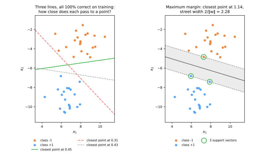
The three lines on the left are all perfect on training, but each one passes within just 0.31 to 0.45 of some point: a new point only slightly different from that one could land on the wrong side. The maximum-margin line on the right keeps every training point at least 1.14 away, so the street between the dashed lines is 2.28 wide. The circled points sit exactly on the edges of the street. They are the support vectors: the solution depends on them and on nothing else.
2. The geometry, by hand
Distance to a hyperplane
Stage 2. For a hyperplane \(w^\top x + b = 0\), the distance from a point \(x\) to it is
Multiplying \(w\) and \(b\) by the same constant does not move the hyperplane, so the SVM fixes the scale: the closest points must have \(\lvert w^\top x + b \rvert = 1\). Those points lie on the two dashed lines \(f(x) = +1\) and \(f(x) = -1\), each at distance \(1/\lVert w \rVert\) from the boundary, so the street is \(2 / \lVert w \rVert\) wide. Maximizing the street is the same as minimizing \(\lVert w \rVert\):
This is a convex quadratic program: one global optimum, no random initialization, no learning rate.
Numeric example: six points
Take three points of each class:
| point | \(x_1\) | \(x_2\) | \(y\) |
|---|---|---|---|
| A | 0 | 0 | −1 |
| B | 1 | 0 | −1 |
| C | 0 | 1 | −1 |
| D | 2 | 2 | +1 |
| E | 3 | 2 | +1 |
| F | 2 | 3 | +1 |
By hand. The two groups face each other along the diagonal, so by symmetry the best boundary is perpendicular to it: \(w = (a, a)\), a line \(x_1 + x_2 = \text{const}\). The closest negative points are B and C (\(x_1 + x_2 = 1\)); the closest positive point is D (\(x_1 + x_2 = 4\)). The boundary goes halfway, at \(x_1 + x_2 = 2.5\). The scale condition says \(f = +1\) at D and \(f = -1\) at B:
So \(w = (0.667, 0.667)\), \(\lVert w \rVert = \tfrac{2}{3}\sqrt{2} = 0.943\), and the street is \(2 / 0.943 = 2.121\) wide — exactly the distance between the lines \(x_1 + x_2 = 1\) and \(x_1 + x_2 = 4\), which is \(3/\sqrt2\).
The library confirms. A hard margin (no violations allowed) is SVC(kernel='linear') with a huge C; why C will become clear in the next section:
import numpy as np
import pandas as pd
from sklearn.svm import SVC

X = np.array([[0, 0], [1, 0], [0, 1], [2, 2], [3, 2], [2, 3]])
y = np.array([-1, -1, -1, 1, 1, 1])

svm = SVC(kernel='linear', C=1e6, tol=1e-8).fit(X, y)     # huge C = hard margin
w, b = svm.coef_[0], svm.intercept_[0]
print("w =", w.round(3), "  b =", round(b, 3))
print("support vectors:", svm.support_, "->", X[svm.support_].tolist())
print(f"street width 2/||w|| = {2 / np.linalg.norm(w):.3f}")
w = [0.667 0.667]   b = -1.667
support vectors: [1 2 3] -> [[1, 0], [0, 1], [2, 2]]
street width 2/||w|| = 2.121
Same \(w\), same \(b\), same width, and the support vectors are rows 1, 2 and 3: B, C and D, the three points on the edges of the street. The score and distance of every point:
f = X @ w + b                                  # the same as svm.decision_function(X)
print(pd.DataFrame({'point': list('ABCDEF'), 'y': y, 'f(x)': f.round(3),
                    'm = y·f(x)': (y * f).round(3),
                    'distance': (np.abs(f) / np.linalg.norm(w)).round(3)}).to_string(index=False))
point  y   f(x)  m = y·f(x)  distance
    A -1 -1.667       1.667     1.768
    B -1 -1.000       1.000     1.061
    C -1 -1.000       1.000     1.061
    D  1  1.000       1.000     1.061
    E  1  1.667       1.667     1.768
    F  1  1.667       1.667     1.768
The support vectors have \(m = 1\) exactly and sit at distance \(1.061\), half the street. A, E and F have \(m > 1\): they are further away than they need to be, and the solution does not care about them.
Only the support vectors matter
The solver actually works on a different but equivalent problem (the dual), with one weight \(\alpha_i \geq 0\) per training point, and rebuilds \(w\) from them:
Points beyond the margin end up with \(\alpha_i = 0\). scikit-learn stores the nonzero products \(\alpha_i y_i\) in dual_coef_:
print("alpha_i * y_i of the support vectors:", svm.dual_coef_.round(3))
print("w rebuilt from them:", (svm.dual_coef_ @ svm.support_vectors_).round(3))
\(w = -\tfrac{2}{9}(1, 0) - \tfrac{2}{9}(0, 1) + \tfrac{4}{9}(2, 2) = (\tfrac{2}{3}, \tfrac{2}{3})\). Three points out of six carry the whole model. The practical consequence: deleting a point that is not a support vector changes nothing, deleting a support vector changes the answer.
for drop, label in [(4, 'E = (3, 2), not a support vector'), (3, 'D = (2, 2), a support vector')]:
    keep = np.arange(len(X)) != drop
    s = SVC(kernel='linear', C=1e6, tol=1e-8).fit(X[keep], y[keep])
    print(f"without {label}: w = {s.coef_[0].round(3)}, b = {s.intercept_[0]:.3f}, "
          f"width {2 / np.linalg.norm(s.coef_):.3f}")
without E = (3, 2), not a support vector: w = [0.667 0.667], b = -1.667, width 2.121
without D = (2, 2), a support vector: w = [0.5 0.5], b = -1.500, width 2.828
Without D, the closest positive points are E and F (\(x_1 + x_2 = 5\)), the street widens to \(4/\sqrt2 = 2.828\) and the boundary moves to \(x_1 + x_2 = 3\). Logistic regression behaves differently: every training point has a nonzero weight in its solution, so removing any point moves its boundary a little.
3. Soft margin and C
Slack and the hinge loss
Stage 3. Real classes overlap, and then no street is empty. The soft margin lets point \(i\) violate its margin by a slack \(\xi_i \geq 0\) and charges for it:
The cheapest slack is \(\xi_i = \max(0,\, 1 - m_i)\), with \(m_i = y_i f(x_i)\). That function has a name, the hinge loss, and substituting it gives the SVM as "loss + penalty":
Put it next to what scikit-learn's LogisticRegression minimizes (L2 penalty):
Same template, same \(C\) in the same place: a large \(C\) makes errors expensive relative to \(\lVert w \rVert\) (weak regularization), a small \(C\) makes them cheap (strong regularization). This is the same inverse regularization you tuned for logistic regression in cross-validation, and the same "loss + penalty" template as Ridge. The only difference between the two classifiers is the loss.
Numeric example: four points against the six-point solution
Keep \(w = (0.667, 0.667)\), \(b = -1.667\) from the hand example and score four new points of class \(+1\):
pts = np.array([[3, 3], [2, 2], [1.5, 1.5], [1, 0.5]])
m = +1 * (pts @ w + b)                                     # y = +1 for all four
print(pd.DataFrame({'point': ['(3, 3)', '(2, 2)', '(1.5, 1.5)', '(1, 0.5)'],
                    'm = y·f(x)': m.round(3),
                    'hinge': np.maximum(0, 1 - m).round(3),
                    'log loss': np.log1p(np.exp(-m)).round(3),
                    '0-1 loss': (m <= 0).astype(int)}).to_string(index=False))
     point  m = y·f(x)  hinge  log loss  0-1 loss
    (3, 3)       2.333  0.000     0.093         0
    (2, 2)       1.000  0.000     0.313         0
(1.5, 1.5)       0.333  0.667     0.540         0
  (1, 0.5)      -0.667  1.667     1.081         1
Check the first and third rows with a calculator: \(f(3,3) = \tfrac{2}{3} \cdot 6 - \tfrac{5}{3} = \tfrac{7}{3} = 2.333\), hinge \(\max(0, 1 - 2.333) = 0\); \(f(1.5, 1.5) = \tfrac{2}{3} \cdot 3 - \tfrac{5}{3} = \tfrac{1}{3}\), hinge \(1 - 0.333 = 0.667\). Four situations:
- (3, 3), well beyond the margin: hinge 0. Log loss is small (0.093) but not zero, so logistic regression still "listens" to this point;
- (2, 2), exactly on the margin: hinge still 0;
- (1.5, 1.5), correct side but inside the street: hinge 0.667 although the 0-1 loss says "correct";
- (1, 0.5), wrong side: hinge 1.667, growing linearly with the distance.
The figure shows the three losses as functions of \(m\), with the four points marked (figure script):
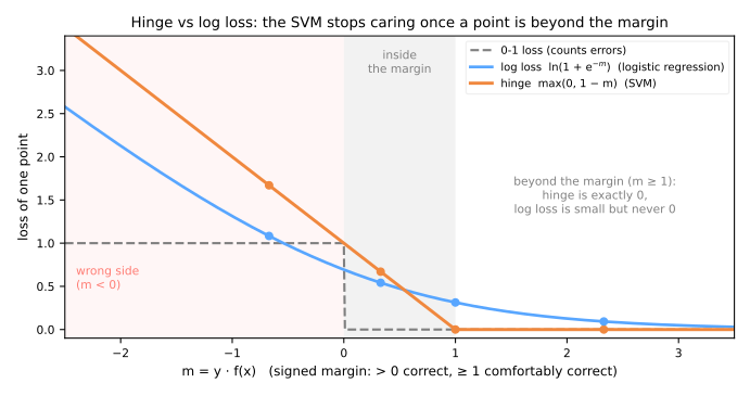
Both losses are convex; that is why both can be optimized reliably. The hinge is also an upper bound of the 0-1 loss: it never charges less than the error count. The log loss, written here with the natural logarithm, is not quite one: on the wrong side and close to the boundary (\(-0.54 < m \leq 0\)) it costs less than 1, as the figure shows; in base 2, \(\log_2(1 + e^{-m})\), it would be. The flat part of the hinge is where the SVM gets its sparsity: points with \(m > 1\) contribute nothing to the loss and get \(\alpha_i = 0\).
What C does, measured
On 100 points from two overlapping clouds, fit a linear SVM for several values of \(C\):
from sklearn.datasets import make_blobs
from sklearn.model_selection import StratifiedKFold, cross_val_score

X, y = make_blobs(n_samples=100, centers=2, cluster_std=1.6, random_state=7)
cv = StratifiedKFold(n_splits=5, shuffle=True, random_state=0)
for C in [0.001, 0.01, 0.1, 1, 100]:
    svm = SVC(kernel='linear', C=C).fit(X, y)
    width = 2 / np.linalg.norm(svm.coef_)
    acc = cross_val_score(SVC(kernel='linear', C=C), X, y, cv=cv).mean()
    print(f"C = {C:<6g} width {width:5.2f} · support vectors {svm.n_support_.sum():3d} · "
          f"train {svm.score(X, y):.2f} · CV {acc:.3f}")
C = 0.001  width  9.23 · support vectors  78 · train 0.99 · CV 1.000
C = 0.01   width  5.13 · support vectors  27 · train 1.00 · CV 0.990
C = 0.1    width  2.63 · support vectors  12 · train 1.00 · CV 1.000
C = 1      width  1.33 · support vectors   6 · train 1.00 · CV 0.990
C = 100    width  0.39 · support vectors   3 · train 1.00 · CV 0.990
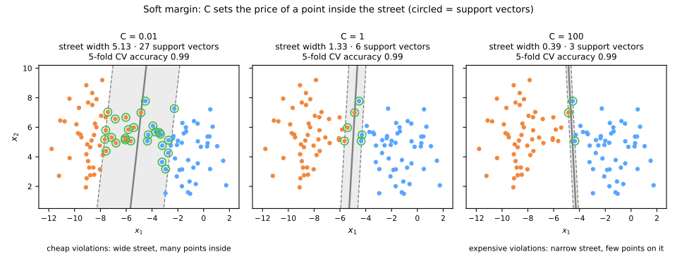
Read the table from top to bottom:
- small \(C\): violations are cheap, so the optimizer prefers a small \(\lVert w \rVert\), that is, a wide street. Many points fall inside it, and every one of them is a support vector (78 of 100 at \(C = 0.001\));
- large \(C\): violations are expensive. The street shrinks until almost no point is inside it: at \(C = 100\) it is 0.39 wide and hangs on 3 points. A hard margin is the limit \(C \to \infty\), which is why the hand example used \(C = 10^6\).
The number of support vectors is a direct readout of how regularized the model is. On this easy problem the cross-validated accuracy barely moves (0.99–1.00), so the geometry changes a lot and the score does not; on harder data, as you will see with kernels, the wrong \(C\) costs real accuracy. \(C\) is a hyperparameter, chosen with cross-validation like the C of logistic regression.
Try it yourself. The simulator solves the soft-margin problem live; slide \(C\) and drag points:
Key idea
The SVM is "loss + penalty" like Ridge, with the hinge loss in place of the log loss. The flat part of the hinge — exactly zero cost for \(m > 1\) — is where sparsity comes from: well-classified points get \(\alpha_i = 0\) and vanish from the solution.
4. Summary: the linear SVM in five lines
- The margin is the ruler. Among all separating lines, take the one furthest from the nearest point: the street of width \(2 / \lVert w \rVert\).
- Maximizing the street = minimizing \(\lVert w \rVert\), subject to \(y_i f(x_i) \geq 1\). It is a convex quadratic program: one global optimum, no learning rate.
- Only the support vectors matter. \(w = \sum_i \alpha_i y_i x_i\), and \(\alpha_i = 0\) for every point beyond the margin.
- The soft margin charges \(C\) per unit of violation; the cheapest slack is the hinge loss \(\max(0, 1 - m)\).
- \(C\) is the same knob as in logistic regression: small = strong regularization = wide street = many support vectors.
| symptom | what is happening | what to do |
|---|---|---|
| almost every point is a support vector | \(C\) too small: the street swallowed the data | raise \(C\) |
| 2 or 3 support vectors and training accuracy 1.00 | \(C\) too large: an almost hard margin | lower \(C\); look at CV, not training |
| huge or tiny scores | features on different scales | StandardScaler inside the pipeline |
| the linear boundary does not fit | the problem is not linearly separable | the kernel, in the advanced part |
Fundamental lab — the linear SVM
The problem. The Ionosphere dataset (Sigillito et al., 1989) comes from a radar array in Goose Bay, Labrador, that sends pulses into the ionosphere. Each of the 351 rows is one return, described by 34 numbers (17 pulse measurements, each a pair of values of the complex autocorrelation function). A "good" return (g) shows evidence of structure in the ionosphere; a "bad" one (b) passes through it. The task: classify returns automatically. It is a small, high-dimensional problem with a nonlinear boundary, the kind of problem where kernels matter.
The workflow is the one from the validation lesson: lock a test set away, compare models on the same cross-validation folds, and touch the test exactly once, in step 9.
How to run this lab in class (about 30 min, in pairs)
- Open the lab notebook on Colab (in Portuguese). There is nothing to download or install: Colab runs in the browser. To keep your answers, save a copy to your Drive (File → Save a copy in Drive) before editing. Run the cells in order, in one session.
- This lab covers steps 1 to 4 of the notebook. The advanced lab continues in the same notebook, from step 5.
- Each step starts with a Predict: answer it with your partner before running the cell. Getting the prediction wrong is what makes the result stick.
- After running, compare with the output and the reading on this page. Every output here is exactly what the code prints.
- The Simulations ask you to write a small Python experiment: change one input and watch what happens to the output. No arithmetic by hand. The solution is collapsed right below: try before opening it.
- Suggested pace: steps 1 to 3 in 10 min; step 4 and the two simulations in 20 min.
Step 1 — load and look
Predict. Before running: for an SVM, what matters most about the 34 columns — their means, their range of values, or how many are categorical? Why?
import numpy as np
import pandas as pd
from sklearn.datasets import fetch_openml

data = fetch_openml(data_id=59, as_frame=True)       # Ionosphere (UCI)
X = data.data                                        # 34 numeric features
y = (data.target == 'g').astype(int)                 # 1 = "good" radar return, 0 = "bad"
print(X.shape)
print(y.value_counts())
print(f"values from {X.min().min():.0f} to {X.max().max():.0f} · "
      f"constant columns: {list(X.columns[X.std() == 0])}")
(351, 34)
class
1    225
0    126
Name: count, dtype: int64
values from -1 to 1 · constant columns: ['a02']
351 returns: 225 good (64.1%) and 126 bad. Two details matter for an SVM. First, every value already lies between −1 and 1 (the features are normalized autocorrelation values, and a01 is a 0/1 flag), so the scales are comparable even before any preprocessing; we still standardize inside the pipeline, which costs nothing and makes every feature's variance 1. Second, column a02 is zero in every row. It carries no information, and it is harmless: StandardScaler leaves a constant column at 0, so it adds nothing to any distance or kernel.
Step 2 — lock the test set away
Predict. With 88 test rows, how much is a single row worth in accuracy points? Does that change how much you should trust the third decimal of the final number?
from sklearn.model_selection import train_test_split

X_train, X_test, y_train, y_test = train_test_split(
    X, y, test_size=0.25, stratify=y, random_state=42)
print(X_train.shape, X_test.shape)
print(f"share of 'good': train {y_train.mean():.3f} · test {y_test.mean():.3f}")
263 rows for development and 88 locked away until step 9, both with the same 64% share of good returns thanks to stratify=y. With 88 test rows, a single row is worth 1.14 points of accuracy; keep that in mind when you read the final number.
Step 3 — a baseline and the folds everyone shares
Predict. What percentage does always answering "good" get right? And what will that baseline's ROC AUC be?
from sklearn.dummy import DummyClassifier
from sklearn.model_selection import StratifiedKFold, cross_validate

cv = StratifiedKFold(n_splits=5, shuffle=True, random_state=42)


def cv_summary(model):
    r = cross_validate(model, X_train, y_train, cv=cv, scoring=['accuracy', 'roc_auc'])
    return {metric: f"{r['test_' + metric].mean():.3f} ± {r['test_' + metric].std():.3f}"
            for metric in ['accuracy', 'roc_auc']}


print(cv_summary(DummyClassifier(strategy='most_frequent')))
Always answering "good" is right 64.3% of the time, and its ROC AUC is 0.5 because it ranks nothing. Any accuracy must be read against 0.643, not against 0.5. The cv object is created once and reused by every later step, so all models are scored on the same five folds and their differences come from the models, not from the luck of the split. cv_summary reports the mean ± standard deviation over the five folds.
Step 4 — three models you know, on the same folds
Predict. Logistic regression and the linear SVM both draw a hyperplane on the same 34 standardized features and differ only in the loss. Do you expect a large gap between them, or one smaller than the between-fold std?
from sklearn.linear_model import LogisticRegression
from sklearn.neighbors import KNeighborsClassifier
from sklearn.pipeline import make_pipeline
from sklearn.preprocessing import StandardScaler
from sklearn.svm import SVC

models = {
    'logistic regression': make_pipeline(StandardScaler(), LogisticRegression(max_iter=1000)),
    'k-NN (k = 5)': make_pipeline(StandardScaler(), KNeighborsClassifier()),
    'linear SVM (C = 1)': make_pipeline(StandardScaler(), SVC(kernel='linear')),
}
print(pd.DataFrame({name: cv_summary(m) for name, m in models.items()}).T)
                          accuracy        roc_auc
logistic regression  0.882 ± 0.021  0.895 ± 0.044
k-NN (k = 5)         0.818 ± 0.025  0.901 ± 0.031
linear SVM (C = 1)   0.886 ± 0.017  0.850 ± 0.052
How to read it:
- Logistic regression and the linear SVM tie on accuracy (0.882 vs 0.886, a difference far smaller than either standard deviation). Both draw a hyperplane in the same 34 standardized features; they only disagree on the loss, and here that barely matters.
- The linear SVM's ROC AUC is lower (0.850 ± 0.052 vs 0.895 ± 0.044), but the gap is about one fold standard deviation: suggestive, not conclusive.
- k-NN has the worst accuracy (0.818) and the best ROC AUC of the three (0.901). Its ranking of the returns is good, its default decision (majority of 5 neighbors) is not. A local model sees something the two linear ones miss, which is a hint that the boundary is not a hyperplane.
Simulation: only the support vectors matter. Section 2 claimed that deleting a point that is not a support vector changes nothing. Test it on the lab's data: standardize once (to isolate the effect, since a refit scaler would change everything), fit a linear SVM, find which rows are support vectors, and refit without one row of each kind. What happens to \(\lVert w \rVert\)?
Solution
Z = StandardScaler().fit_transform(X_train)   # standardize ONCE, to isolate the effect
lin = SVC(kernel='linear').fit(Z, y_train)
sv = set(lin.support_)
print(f"{len(sv)} support vectors of {len(Z)} rows")

for label, drop in [('a non-support-vector row', next(i for i in range(len(Z)) if i not in sv)),
                    ('a support vector', lin.support_[0])]:
    keep = np.arange(len(Z)) != drop
    s = SVC(kernel='linear').fit(Z[keep], y_train.iloc[keep])
    print(f"without {label:24s}: ||w|| {np.linalg.norm(s.coef_):.6f} "
          f"(was {np.linalg.norm(lin.coef_):.6f}) · support vectors {s.n_support_.sum()}")
70 support vectors of 263 rows
without a non-support-vector row: ||w|| 3.808782 (was 3.808803) · support vectors 70
without a support vector        : ||w|| 3.767861 (was 3.808803) · support vectors 70
Deleting one of the 193 rows that are not support vectors leaves \(\lVert w \rVert\) practically unchanged: the difference, 0.00002, is solver tolerance, not a different model. Deleting one support vector already moves the second decimal (3.7679 against 3.8088), a difference about two thousand times larger. The solution depends on 70 points out of 263 and is literally indifferent to the other 193 — which logistic regression is not, because there every point carries a non-zero weight. Note too that standardizing once was essential to the test: inside a pipeline, removing any row also changes the scaler's means and standard deviations, and then everything shifts a little.
Simulation: C changes the width of the street. Sweep the linear SVM's C from 0.01 to 100 and measure, for each value, the street width \(2/\lVert w \rVert\), how many support vectors are left, the training accuracy and the cross-validated one. Where does CV peak, and what happens to it afterwards?
Solution
from sklearn.model_selection import cross_val_score

for C in [0.01, 0.1, 1, 10, 100]:
    m = make_pipeline(StandardScaler(), SVC(kernel='linear', C=C)).fit(X_train, y_train)
    width = 2 / np.linalg.norm(m[-1].coef_)
    acc = cross_val_score(make_pipeline(StandardScaler(), SVC(kernel='linear', C=C)),
                          X_train, y_train, cv=cv).mean()
    print(f"C = {C:<6g} street {width:6.3f} · support vectors {m[-1].n_support_.sum():3d}"
          f" · train {m.score(X_train, y_train):.3f} · CV {acc:.3f}")
C = 0.01   street  2.979 · support vectors 137 · train 0.886 · CV 0.863
C = 0.1    street  1.219 · support vectors  96 · train 0.913 · CV 0.871
C = 1      street  0.525 · support vectors  70 · train 0.947 · CV 0.886
C = 10     street  0.256 · support vectors  58 · train 0.954 · CV 0.871
C = 100    street  0.135 · support vectors  50 · train 0.962 · CV 0.852
The street shrinks 22-fold from end to end and the support vectors fall from 137 to 50, exactly as section 3 predicted. What the lesson's toy example did not show appears here: training accuracy climbs without stopping (0.886 → 0.962) while cross-validated accuracy traces an arc, peaking at C = 1 (0.886) and dropping to 0.852 at C = 100. That is the signature of overfitting, and it is why \(C\) is chosen on CV and not on training. Note in passing that even the best value stays far below the 0.939 the RBF kernel reaches with no tuning at all in step 5: here the problem is not \(C\), it is the straight line.
To close the fundamental part. One sentence each: (1) why can training accuracy not choose between two separating lines? (2) What changes in the solution if you delete a point beyond the margin? (3) What does a small \(C\) do to the street width and to the number of support vectors?
Your turn (fundamental)
For homework:
- The margin by hand. Take the six points of section 2 and move D from (2, 2) to (2.5, 2.5). Redo the computation by hand (the boundary is still perpendicular to the diagonal) and check it with
SVC(kernel='linear', C=1e6). Did the street get wider or narrower? - Hinge against log loss. For \(m\) from −3 to 3, plot
np.maximum(0, 1 - m)andnp.log1p(np.exp(-m)). Where do they cross? Which of the two punishes a gross error more, and which keeps "listening" to a well-classified point? - How many support vectors? In the lab, redo the \(C\) simulation with
kernel='linear'onload_breast_cancer. Is the relationship between \(C\) and the number of support vectors the same? And does the CV curve trace a similar arc?
Advanced approach
The fundamental part left a linear machine with one knob. This part answers how it draws curved boundaries without ever leaving the linear world — the kernel trick — and what that charges: a second hyperparameter coupled to the first, mandatory scaling, no native probabilities, and a training cost that grows at least like \(n^2\). The code blocks continue those of sections 1 to 3.
This part follows one pipeline in four stages: 1. the kernel trick, curved boundaries from a linear machine; 2. tune C and γ, two coupled knobs and mandatory scaling; 3. read the output, scores, probabilities and multiclass; 4. when to use it, training cost and the practical profile. Each stage links to its section, and in the slides a strip at the bottom shows which stage you are in.
- The kernel trickfeature maps, the kernel, RBF (radial basis function)
- Tune C and γtwo coupled knobs; scaling is mandatory
- Read the outputscores, probabilities, multiclass
- When to use ittraining cost, the practical profile
Slides: advanced approach
Click the slides and use the ← → arrows to navigate; F goes full screen and Esc shows every slide. Open the slides in a new tab
5. The kernel trick
A feature map makes data separable
Stage 1. Some classes are not separable by any line in the features you have. Twelve points on a line, the outer ones \(+1\) and the inner ones \(-1\):
x = np.array([-3.0, -2.6, -2.1, -1.2, -0.7, -0.2, 0.3, 0.9, 1.3, 2.0, 2.4, 2.9])
y = np.where(np.abs(x) > 1.6, 1, -1)                     # outer points +1, inner points -1

cuts = np.r_[x.min() - 1, (x[:-1] + x[1:]) / 2, x.max() + 1]
best_cut = max(np.mean(np.where(x > t, s, -s) == y) for t in cuts for s in [1, -1])
print(f"best single threshold on x: {best_cut:.2f} accuracy")

Phi = np.c_[x, x ** 2]                                   # the feature map x -> (x, x²)
svm = SVC(kernel='linear', C=1e6, tol=1e-8).fit(Phi, y)
(w1, w2), b = svm.coef_[0], svm.intercept_[0]
print(f"linear SVM on (x, x²): {svm.score(Phi, y):.2f} accuracy")
print("the line w1·x + w2·x² + b = 0 crosses x at", np.sort(np.roots([w2, w1, b])).round(2))
best single threshold on x: 0.75 accuracy
linear SVM on (x, x²): 1.00 accuracy
the line w1·x + w2·x² + b = 0 crosses x at [-1.79  1.69]
No threshold on \(x\) gets more than 9 of the 12 points right. Add one column, \(x^2\), and a plain linear SVM separates them perfectly (figure script):
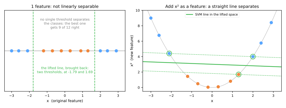
A line in the new space \((x, x^2)\) is a parabola condition in the old one, \(w_1 x + w_2 x^2 + b > 0\), and here it becomes two thresholds, at −1.79 and 1.69. This is exactly the idea of polynomial features: a linear model in a richer feature space is a nonlinear model in the original one.
The catch is size. With \(d\) features, all monomials up to degree \(p\) number \(\binom{d+p}{p}\):
from math import comb

for d, p in [(2, 2), (34, 3), (784, 3)]:
    print(f"d = {d:3d}, degree {p}: {comb(d + p, p):>11,} monomials")
d =   2, degree 2:           6 monomials
d =  34, degree 3:       7,770 monomials
d = 784, degree 3:  80,931,145 monomials
With 784 pixels (a 28 × 28 image) and degree 3, the explicit map has over 80 million columns.
The kernel: an inner product without the map
The dual problem and the prediction touch the data only through inner products \(x_i^\top x_j\):
So if we map \(x \to \phi(x)\), all we ever need is \(\langle \phi(x_i), \phi(x_j) \rangle\). A kernel is a function that returns that number directly from the original vectors:
Numeric check, degree-2 polynomial kernel. For two features, \(\phi(v) = (v_1^2,\ \sqrt2\, v_1 v_2,\ v_2^2)\). Take \(u = (1, 2)\) and \(v = (3, 1)\):
- through the map: \(\phi(u) = (1,\ 2\sqrt2,\ 4)\), \(\phi(v) = (9,\ 3\sqrt2,\ 1)\), so \(\phi(u) \cdot \phi(v) = 9 + 12 + 4 = 25\);
- through the kernel: \(u \cdot v = 3 + 2 = 5\), and \(K(u, v) = (u \cdot v)^2 = 25\).
from sklearn.metrics.pairwise import polynomial_kernel

u, v = np.array([1.0, 2.0]), np.array([3.0, 1.0])
phi = lambda z: np.array([z[0] ** 2, np.sqrt(2) * z[0] * z[1], z[1] ** 2])
print("phi(u)·phi(v) =", round(phi(u) @ phi(v), 6))
print("(u·v)^2       =", (u @ v) ** 2)
print("scikit-learn  =", polynomial_kernel([u], [v], degree=2, gamma=1, coef0=0)[0, 0])
The kernel costs one 2-term dot product and a square, however many monomials the map has. That is the kernel trick: linear machinery (margin, hinge, support vectors) in a huge feature space, at the cost of computing \(K\) between pairs of points in the original space.
| Kernel | \(K(u, v)\) | Notes |
|---|---|---|
| linear | \(u^\top v\) | the SVM of the fundamental part; best for high-dimensional sparse data (text) |
| polynomial | \((\gamma\, u^\top v + r)^p\) | all feature interactions up to degree \(p\); coef0 \(= r\) |
| RBF (Gaussian) | \(\exp(-\gamma \lVert u - v \rVert^2)\) | the default; its feature space is infinite-dimensional |
One detail of the polynomial kernel: scikit-learn's default coef0=0 keeps only the terms of degree exactly \(p\) (as in the check above). With coef0=1 all lower degrees are included as well, which is what you usually want.
The RBF kernel is a similarity
The RBF kernel equals 1 when \(u = v\) and decays toward 0 with distance; \(\gamma\) sets how fast. Three points on a line, at 0, 1 and 3:
from sklearn.metrics.pairwise import rbf_kernel

P = np.array([[0.0, 0.0], [1.0, 0.0], [3.0, 0.0]])
for gamma in [0.1, 0.5, 2]:
    K = rbf_kernel(P, gamma=gamma)
    print(f"gamma = {gamma:<3}: K(0, 1) = {K[0, 1]:.3f} · K(0, 3) = {K[0, 2]:.5f}")
gamma = 0.1: K(0, 1) = 0.905 · K(0, 3) = 0.40657
gamma = 0.5: K(0, 1) = 0.607 · K(0, 3) = 0.01111
gamma = 2  : K(0, 1) = 0.135 · K(0, 3) = 0.00000
By hand for \(\gamma = 0.5\): \(e^{-0.5 \cdot 1} = 0.607\) and \(e^{-0.5 \cdot 9} = 0.011\). With \(\gamma = 0.1\), a point 3 units away still counts as quite similar (0.407); with \(\gamma = 2\), even a point 1 unit away barely counts (0.135) and one 3 units away does not count at all.
Now read the prediction again with this kernel:
It is a weighted vote of the support vectors near \(x\): each one votes for its class \(y_i\), with a weight that fades with distance. That is k-NN with two changes: the vote is smooth instead of "the k closest, equally", and only the support vectors vote, with weights \(\alpha_i\) learned by the margin optimization. \(\gamma\) plays a role similar to \(1/k\): large \(\gamma\) means only very close points matter.
Kernels compared, measured
Two datasets no line can separate, three kernels, 5-fold CV:
from sklearn.datasets import make_circles, make_moons
from sklearn.pipeline import make_pipeline
from sklearn.preprocessing import StandardScaler

datasets = {'circles': make_circles(n_samples=200, factor=0.4, noise=0.12, random_state=0),
            'moons': make_moons(n_samples=200, noise=0.25, random_state=0)}
kernels = {'linear': SVC(kernel='linear'),
           'poly, degree 3': SVC(kernel='poly', degree=3, coef0=1),
           'RBF': SVC(kernel='rbf')}
table = {dname: {kname: cross_val_score(make_pipeline(StandardScaler(), k), Xd, yd, cv=cv).mean()
                 for kname, k in kernels.items()}
         for dname, (Xd, yd) in datasets.items()}
print(pd.DataFrame(table).round(3))
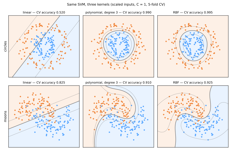
On the circles the linear SVM is at chance (0.520): no line helps. Both nonlinear kernels draw the ring. On the moons the linear kernel still gets 0.825 (a line captures the rough trend), and the RBF kernel reaches 0.925 by following the curved gap. The RBF kernel is the default in scikit-learn because it rarely does badly; the linear kernel remains the right first try when there are many features, as in text.
6. C and γ together
Stage 2. With the RBF kernel there are two hyperparameters, and they interact:
- \(\gamma\) is the reach of each support vector. Small \(\gamma\): every support vector influences a wide region, and the boundary is almost linear. Large \(\gamma\): each support vector influences only its immediate neighborhood, and the boundary can wrap individual points;
- \(C\) is, as before, the price of a margin violation.
They are tuned together on a logarithmic grid, with a scaler in a pipeline and cross-validation, exactly the procedure of the validation lesson:
from sklearn.model_selection import GridSearchCV

X, y = make_moons(n_samples=300, noise=0.3, random_state=1)
grid = GridSearchCV(make_pipeline(StandardScaler(), SVC()),
                    {'svc__C': [0.01, 0.1, 1, 10, 100, 1000],
                     'svc__gamma': [0.01, 0.1, 1, 10, 100, 1000]}, cv=cv)
grid.fit(X, y)
res = pd.DataFrame(grid.cv_results_)
print(res.pivot(index='param_svc__C', columns='param_svc__gamma', values='mean_test_score').round(3))
print(grid.best_params_, f"CV accuracy {grid.best_score_:.3f} ± {res.loc[grid.best_index_, 'std_test_score']:.3f}")
param_svc__gamma  0.01     0.10     1.00     10.00    100.00   1000.00
param_svc__C
0.01                0.830    0.837    0.863    0.897    0.723    0.550
0.10                0.830    0.837    0.870    0.897    0.723    0.550
1.00                0.843    0.837    0.920    0.897    0.840    0.570
10.00               0.830    0.857    0.917    0.877    0.823    0.583
100.00              0.833    0.890    0.903    0.860    0.823    0.583
1000.00             0.837    0.913    0.903    0.860    0.823    0.583
{'svc__C': 1, 'svc__gamma': 1} CV accuracy 0.920 ± 0.022
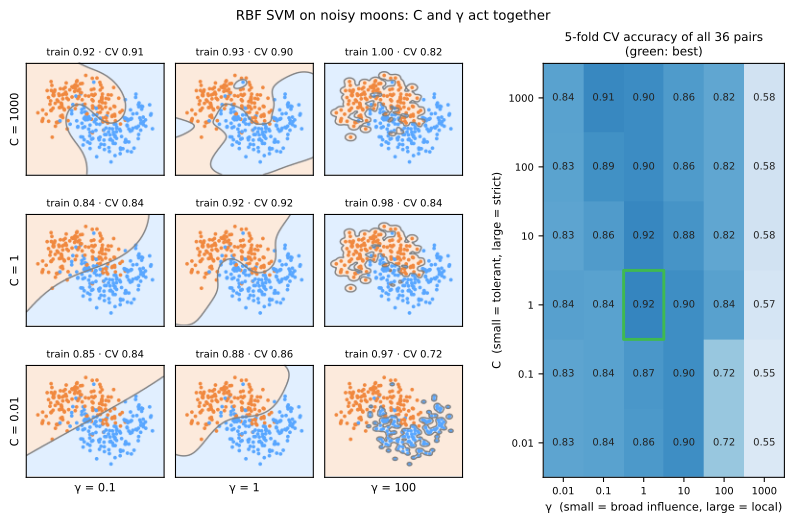
Three regions to recognize, in the table and in the picture:
- Underfitting (left columns, \(\gamma = 0.01\)): every support vector reaches the whole plane, so the boundary is nearly a straight line, and accuracy is stuck at 0.83–0.84 for every \(C\). The bottom-left panel (\(C = 0.01\), \(\gamma = 0.1\)) is essentially the linear SVM.
- Overfitting (right-hand column of the table, \(\gamma = 1000\); in the panels, the \(\gamma = 100\) column): every support vector is an island. Training accuracy is already 0.97–1.00 at \(\gamma = 100\) (right column of panels), but a new point is far from every island, gets \(f(x) \approx b\), and falls into one class; CV accuracy collapses to 0.55–0.58, barely above the 50% baseline. At \(\gamma = 100\) with small \(C\), the panel shows the islands around one class.
- The good diagonal: the best cells form a ridge running from large \(C\) with small \(\gamma\) (0.913 at \(C = 1000\), \(\gamma = 0.1\)) through the winner (0.920 at \(C = 1\), \(\gamma = 1\)) to small \(C\) with larger \(\gamma\) (0.897 at \(C \leq 1\), \(\gamma = 10\)). Both knobs trade flexibility for smoothness, so a little less of one can be compensated by a little more of the other. This is why they must be searched together: tuning \(C\) at a fixed, badly chosen \(\gamma\) finds only the best cell of a bad column.
As in the validation lesson, read the winner with its noise: its fold standard deviation is 0.022, and every cell from 0.898 up (0.917, 0.913, 0.903, …) is within one standard deviation of it. "\(C = 1, \gamma = 1\)" is a fine choice, not a proven optimum.
7. Scaling is mandatory
The RBF kernel measures squared Euclidean distance, and so does the margin: a feature measured in thousands dominates one measured in fractions, exactly as in k-NN. Measured on two datasets whose features have very different spreads, with and without a StandardScaler in the pipeline:
from sklearn.datasets import load_breast_cancer, load_wine

for name, loader in [('wine', load_wine), ('breast cancer', load_breast_cancer)]:
    Xd, yd = loader(return_X_y=True)
    raw = cross_val_score(SVC(), Xd, yd, cv=cv).mean()
    scaled = cross_val_score(make_pipeline(StandardScaler(), SVC()), Xd, yd, cv=cv).mean()
    print(f"{name:13s} feature std from {Xd.std(0).min():.3f} to {Xd.std(0).max():5.1f} · "
          f"raw {raw:.3f} · scaled {scaled:.3f}")
wine          feature std from 0.124 to 314.0 · raw 0.657 · scaled 0.983
breast cancer feature std from 0.003 to 568.9 · raw 0.921 · scaled 0.977
On wine, one feature (proline, in the hundreds) has a standard deviation over 2,500 times that of the smallest one. Unscaled, the kernel sees almost only proline, and accuracy is 0.657; scaled, 0.983. The default gamma='scale' does not fix this: it divides by the variance of all features pooled together, so it adapts \(\gamma\) to the overall scale but not to differences between features. The scaler goes inside the pipeline, so that each CV fold fits its own scaler on its own training rows.
8. Scores and probabilities
decision_function is enough for ROC
Stage 3. An SVM's natural output is the score \(f(x)\), available as decision_function. Its sign is the prediction, and its value is a signed distance to the boundary in units of the half-margin: \(\pm 1\) on the edges of the street. It is not a probability, but it ranks points, and ranking is all that ROC AUC and average precision need.
When you do need probabilities (to combine with costs, or to report a risk), the standard fix is Platt scaling (Platt, 1999): fit a one-feature logistic regression \(P(y = 1 \mid x) = 1 / (1 + e^{A f(x) + B})\) on scores obtained by internal cross-validation, then refit the SVM on all the data. SVC(probability=True) has always done this internally; since scikit-learn 1.9 it is deprecated in favor of the explicit, equivalent CalibratedClassifierCV(..., method='sigmoid', ensemble=False), which works on older versions too:
from sklearn.calibration import CalibratedClassifierCV
from sklearn.metrics import roc_auc_score
from sklearn.model_selection import train_test_split

Xd, yd = load_breast_cancer(return_X_y=True)
X_tr, X_te, y_tr, y_te = train_test_split(Xd, yd, test_size=0.25, stratify=yd, random_state=0)

svm = make_pipeline(StandardScaler(), SVC()).fit(X_tr, y_tr)
platt = CalibratedClassifierCV(make_pipeline(StandardScaler(), SVC()), method='sigmoid',
                               ensemble=False, cv=cv).fit(X_tr, y_tr)
f, p = svm.decision_function(X_te), platt.predict_proba(X_te)[:, 1]
print(f"ROC AUC from f(x): {roc_auc_score(y_te, f):.4f} · from Platt probabilities: {roc_auc_score(y_te, p):.4f}")

near = np.argsort(np.abs(f))[:3]                          # the three test points closest to f = 0
print(pd.DataFrame({'f(x)': f[near].round(3), 'P(y=1)': p[near].round(3),
                    'SVC predicts': svm.predict(X_te[near]), 'Platt predicts': platt.predict(X_te[near])}))
print("disagreements on the test set:", (svm.predict(X_te) != platt.predict(X_te)).sum(), "of", len(y_te))
ROC AUC from f(x): 0.9927 · from Platt probabilities: 0.9927
    f(x)  P(y=1)  SVC predicts  Platt predicts
0 -0.001   0.451             0               0
1  0.043   0.494             1               0
2  0.104   0.554             1               1
disagreements on the test set: 1 of 143
Two things to notice:
- The ROC AUC is identical to four decimals. Platt's sigmoid is monotone, so it preserves the ranking of the scores; the probabilities add calibration, not discrimination. For ROC, precision–recall curves or choosing a threshold on validation scores,
decision_functionis enough and needs no extra fits. - The two can disagree near the boundary. The point with \(f(x) = 0.043\) is class 1 for the SVM (positive score) but gets \(P = 0.494\), class 0 for the calibrated model, because the fitted sigmoid is not centered exactly at \(f = 0\). One test point out of 143 here. It also costs extra fits: 5 internal CV fits plus the final one.
Imbalanced classes: class_weight
class_weight='balanced' multiplies the hinge loss of each point by the inverse frequency of its class, exactly as in the imbalanced-data lesson; for the SVM it means a separate \(C\) per class. Measured on a synthetic problem with 10% positives:
from sklearn.datasets import make_classification
from sklearn.model_selection import cross_validate

Xd, yd = make_classification(n_samples=1000, weights=[0.9], n_features=10, n_informative=4,
                             flip_y=0.03, random_state=0)
for cw in [None, 'balanced']:
    r = cross_validate(make_pipeline(StandardScaler(), SVC(class_weight=cw)), Xd, yd, cv=cv,
                       scoring=['recall', 'precision', 'balanced_accuracy', 'roc_auc'])
    print(f"class_weight={str(cw):9s}", " · ".join(f"{k[5:]} {v.mean():.3f}" for k, v in r.items()
                                                  if k.startswith('test_')))
class_weight=None      recall 0.181 · precision 0.893 · balanced_accuracy 0.589 · roc_auc 0.838
class_weight=balanced  recall 0.578 · precision 0.379 · balanced_accuracy 0.727 · roc_auc 0.809
Recall of the minority class rises from 0.181 to 0.578 and precision falls from 0.893 to 0.379: the same trade-off as moving the threshold, paid for with a model that is refit. The ROC AUC does not improve; it even falls (0.838 to 0.809). Reweighting is not a threshold shift: the model is refit, which moves the boundary in favor of the minority class and can rank the scores slightly worse overall.
9. Multiclass: one-vs-one
The SVM is a two-class method. SVC handles \(k\) classes with one-vs-one: it trains one binary SVM for every pair of classes, \(k(k-1)/2\) of them, and predicts by majority vote. On the 10-digit dataset (8 × 8 images, 64 pixel features):
from sklearn.datasets import load_digits
from sklearn.svm import LinearSVC

Xd, yd = load_digits(return_X_y=True)
ovo = SVC(decision_function_shape='ovo').fit(Xd, yd)
print("pairwise classifiers:", ovo.decision_function(Xd[:1]).shape[1], "= 10·9/2")
print("support vectors per digit:", ovo.n_support_, "· total", ovo.n_support_.sum(), "of", len(Xd))
print("LinearSVC (one-vs-rest) coefficients:", LinearSVC().fit(Xd, yd).coef_.shape)
print(f"CV accuracy · raw pixels {cross_val_score(SVC(), Xd, yd, cv=cv).mean():.3f} · "
      f"scaled {cross_val_score(make_pipeline(StandardScaler(), SVC()), Xd, yd, cv=cv).mean():.3f}")
pairwise classifiers: 45 = 10·9/2
support vectors per digit: [ 45  94  66  78  62  77  52  72 106  95] · total 747 of 1797
LinearSVC (one-vs-rest) coefficients: (10, 64)
CV accuracy · raw pixels 0.987 · scaled 0.981
45 pairwise classifiers, each trained only on the rows of its two digits (about a fifth of the data), which is cheaper than it sounds for a method whose cost grows faster than \(n\). By default predict and decision_function present the result as one column per class (decision_function_shape='ovr'), but underneath it is still one-vs-one. LinearSVC uses one-vs-rest instead: 10 classifiers, one row of 64 coefficients each.
The last line refines "scaling is mandatory": pixels are all in the same unit (0–16 gray levels), so there is nothing to equalize, and standardizing actually costs a little (0.987 raw vs 0.981 scaled), most likely because it inflates near-constant border pixels to the same weight as the informative ones. The rule is "put all features on a comparable scale"; StandardScaler is the usual way, not the only one.
10. Cost: when SVMs stop being practical
Training time
Stage 4. A kernel SVM needs the kernel between pairs of training points, and the number of pairs grows as \(n^2\). In practice, solvers take between about \(n^2\) and \(n^3\) operations, depending on how many points end up as support vectors (figure script):
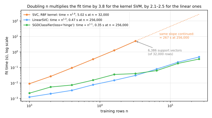
The absolute times depend on the machine that ran the script; the slopes do not. Each doubling of \(n\) multiplies the kernel SVM's fit time by about 3.8 (slope 1.9 on the log-log plot). At 32,000 rows it takes about 5 seconds and keeps over 6,000 support vectors, which also makes prediction slow: every new point needs a kernel evaluation against each one. Continuing the same slope, 256,000 rows would take about 4.5 minutes, for one fit of one \((C, \gamma)\) pair; a 25-cell grid with 5-fold CV multiplies that by 125.
For linear SVMs there are specialized solvers that never form the kernel matrix: LinearSVC (liblinear) and SGDClassifier(loss='hinge'), which minimizes the same hinge + L2 objective by stochastic gradient descent. Both fit 256,000 rows in under half a second in the figure. How close do they get to SVC(kernel='linear')? On the digits:
from sklearn.linear_model import SGDClassifier
from sklearn.multiclass import OneVsOneClassifier, OneVsRestClassifier

linear_models = {'SVC(kernel="linear")': SVC(kernel='linear'),
                 'LinearSVC()': LinearSVC(),
                 'SGDClassifier(hinge)': SGDClassifier(loss='hinge', random_state=0),
                 'SVC, one-vs-rest': OneVsRestClassifier(SVC(kernel='linear')),
                 'LinearSVC, one-vs-one': OneVsOneClassifier(LinearSVC())}
for name, model in linear_models.items():
    acc = cross_val_score(make_pipeline(StandardScaler(), model), Xd, yd, cv=cv).mean()
    print(f"{name:22s} CV accuracy on digits {acc:.3f}")
SVC(kernel="linear")   CV accuracy on digits 0.979
LinearSVC()            CV accuracy on digits 0.955
SGDClassifier(hinge)   CV accuracy on digits 0.949
SVC, one-vs-rest       CV accuracy on digits 0.952
LinearSVC, one-vs-one  CV accuracy on digits 0.979
The specialized solvers land 2–3 points behind (0.955 and 0.949 against 0.979), and the last two rows show that the solver is not the reason. With ten classes, SVC trains one-vs-one (45 pairwise classifiers, section 9), while LinearSVC and SGDClassifier train one-vs-rest: 10 classifiers, each separating one digit from the other nine. Forced into one-vs-rest, SVC drops to 0.952; wrapped in one-vs-one, LinearSVC climbs to 0.979. A straight line separates two digits more easily than one digit from all the others. The remaining differences matter less here: by default LinearSVC uses the squared hinge and also penalizes the intercept, and SGDClassifier makes noisy stochastic passes over the data, with its own regularization parameter alpha instead of C, so each needs its own tuning. What the specialized solvers buy is scale. A rule of thumb from these measurements: a kernel SVM is comfortable up to a few tens of thousands of rows; beyond that, use a linear SVM on well-chosen features, or models that scale better, such as gradient boosting.
How it is trained, in essence
Solvers optimize the dual (e.g. SMO — Sequential Minimal Optimization, Platt 1998 — which optimizes pairs of \(\alpha_i\) until the optimality conditions, called KKT (Karush–Kuhn–Tucker), hold; libsvm, behind SVC, uses a refined version). A pseudocode sketch of the idea:
initialize all α_i = 0
repeat until KKT conditions hold (within tolerance):
    pick a pair (α_i, α_j) violating the conditions      # heuristic choice
    optimize the objective over that pair analytically    # closed form for 2 vars
    clip to 0 ≤ α ≤ C, update b
points ending with α_i > 0 are the support vectors
Regression: SVR
The same ideas give a regressor, SVR: it fits a function with a tube of half-width \(\varepsilon\) around it, ignores residuals smaller than \(\varepsilon\) (the regression analogue of "beyond the margin"), and pays linearly for the rest. Kernels, \(C\), \(\gamma\), scaling and cost behave exactly as in classification.
11. Practical profile
| SVM (RBF kernel) | Logistic regression | k-NN | |
|---|---|---|---|
| Boundary | any smooth shape (kernel) | linear in the features | any shape, local |
| Loss | hinge: ignores points beyond the margin | log loss: every point counts | none (no training) |
| What it stores | the support vectors and their \(\alpha_i\) | \(w, b\) | the whole training set |
| Hyperparameters | \(C\) and \(\gamma\), coupled | \(C\) | \(k\), distance |
| Needs scaling | yes | yes (for the penalty and the solver) | yes |
| Probabilities | no; Platt scaling after the fact | yes, native | vote fractions (coarse) |
| Training cost | \(\sim n^2\) to \(n^3\) | \(\sim n\) | none |
| Prediction cost | one kernel per support vector | one dot product | distances to all \(n\) rows |
| Interpretability | low (except linear kernel) | high: coefficients, odds | medium: "these neighbors" |
| Reach for it when | small/medium \(n\), nonlinear boundary, many features | you need probabilities or explanations, or \(n\) is large | tiny, low-dimensional problems, quick baselines |
Advanced lab — the kernel and the tuning
Steps 5 to 9 switch on the RBF kernel on the same radar problem, tune \(C\) and \(\gamma\) together, open the winner up and measure it exactly once on the test set locked away in step 2.
How to run this lab in class (about 35 min, in pairs)
- Use the same Colab notebook as the fundamental lab and go to step 5 (Passo 5). Nothing to download.
- Steps 5 to 9 use the objects of steps 2 to 4 (
X_train,cv,cv_summary,models). If the Colab session is new (or has expired), click the step 5 cell and use Runtime → Run before (Ctrl+F8) before going on. - Same routine: Predict before running, compare with the page, and try the Simulations before opening the solution.
- Suggested pace: steps 5 and 6 with the simulation in 15 min; step 7 and its simulation in 10 min; steps 8 and 9 in 10 min.
Step 5 — switch on the RBF kernel
Predict. The only change is kernel='rbf', with no tuning at all. Will the gain over the linear SVM be larger or smaller than the between-fold std of step 4 (about 0.02)?
rbf = make_pipeline(StandardScaler(), SVC(kernel='rbf'))       # defaults: C = 1, gamma = 'scale'
print(cv_summary(rbf))

Z = StandardScaler().fit_transform(X_train)
print(f"gamma='scale' means gamma = 1 / (n_features · variance) = {1 / (Z.shape[1] * Z.var()):.4f}")
{'accuracy': '0.939 ± 0.022', 'roc_auc': '0.988 ± 0.007'}
gamma='scale' means gamma = 1 / (n_features · variance) = 0.0303
Switching the kernel from linear to RBF, with no tuning at all, lifts accuracy from 0.886 to 0.939 and ROC AUC from 0.850 to 0.988. The accuracy gain, 5.3 points, is more than twice the fold standard deviation. This is the effect of the kernel, and it is much larger than the differences among the three models of step 4.
The second line decodes gamma='scale'. After standardizing, 33 columns have variance 1 and the constant one has 0, so the pooled variance is \(33/34\) and \(\gamma = 1 / (34 \cdot 33/34) = 1/33 = 0.0303\). A reasonable default, but only a default: step 6 searches around it.
Step 6 — tune C and γ together
Predict. On a grid of 25 \((C, \gamma)\) pairs, do you expect the best \(C\) to depend on the \(\gamma\) chosen? And which corner of the table should be worst: very small or very large \(\gamma\)?
import matplotlib.pyplot as plt
from sklearn.model_selection import GridSearchCV

param_grid = {'svc__C': [0.1, 1, 10, 100, 1000],
              'svc__gamma': [0.0001, 0.001, 0.01, 0.1, 1]}
grid = GridSearchCV(rbf, param_grid, cv=cv, scoring='accuracy', return_train_score=True)
grid.fit(X_train, y_train)

res = pd.DataFrame(grid.cv_results_)
table = res.pivot(index='param_svc__C', columns='param_svc__gamma', values='mean_test_score')
print(table.round(3))
best_std = res.loc[grid.best_index_, 'std_test_score']
print(f"best: {grid.best_params_} · accuracy {grid.best_score_:.3f} ± {best_std:.3f}")
ties = res[res['mean_test_score'] >= grid.best_score_ - best_std]
print(f"{len(ties)} of {len(res)} pairs are within one std of the best")
corner = (res['param_svc__C'] == 1) & (res['param_svc__gamma'] == 1)
print(f"training-fold accuracy · best pair {res.loc[grid.best_index_, 'mean_train_score']:.3f} · "
      f"C = 1, gamma = 1: {res.loc[corner, 'mean_train_score'].item():.3f}")

plt.imshow(table, cmap='Blues', origin='lower')
plt.xticks(range(5), table.columns); plt.yticks(range(5), table.index)
plt.xlabel('gamma'); plt.ylabel('C'); plt.colorbar(label='CV accuracy')
plt.show()
param_svc__gamma  0.0001  0.0010  0.0100  0.1000  1.0000
param_svc__C
0.1                0.643   0.643   0.719   0.643   0.643
1.0                0.643   0.757   0.916   0.954   0.665
10.0               0.753   0.894   0.932   0.951   0.669
100.0              0.878   0.920   0.939   0.954   0.669
1000.0             0.882   0.920   0.932   0.954   0.669
best: {'svc__C': 1, 'svc__gamma': 0.1} · accuracy 0.954 ± 0.019
5 of 25 pairs are within one std of the best
training-fold accuracy · best pair 0.991 · C = 1, gamma = 1: 1.000
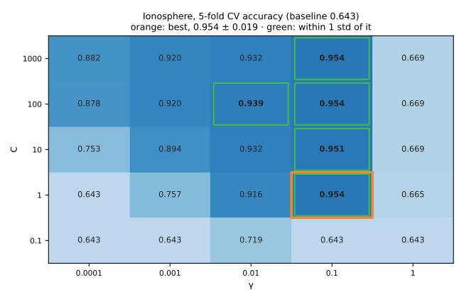
Read the table as a map of three regions:
- Too regularized (first row of the table, \(C = 0.1\), and the \(\gamma = 0.0001\) column at small \(C\)): accuracy 0.643, exactly the baseline, in five of these cells; in the first row only \(\gamma = 0.01\) escapes, and barely (0.719). The margin is so cheap to violate that the SVM gives up and predicts the majority class.
- Too local (right column, \(\gamma = 1\)): 0.665–0.669, barely above the baseline, for every \(C \geq 1\). Each support vector only influences a tiny ball around itself, a new return is far from all of them, gets \(f(x) \approx b\), and is called "good". Meanwhile the training folds are fitted perfectly (1.000 at \(C = 1\), last line of the output, against 0.991 for the winner): the textbook overfitting corner.
- The ridge: the best cells sit at \(\gamma = 0.1\) (and \(\gamma = 0.01\) with large \(C\)).
The winner is \(C = 1\), \(\gamma = 0.1\), with 0.954 ± 0.019. Three cells print 0.954 (\(C\) = 1, 100 and 1000 at \(\gamma = 0.1\)); GridSearchCV keeps the first one it met, which is also the most regularized, a sensible tie-break. Five of 25 pairs are within one standard deviation of the best (green in the figure): four at \(\gamma = 0.1\), with \(C\) anywhere from 1 to 1000, and one at \(\gamma = 0.01\) with \(C = 100\) (0.939). On this dataset, \(\gamma\) is the knob that matters. Note also the size of the gain: tuning moved accuracy from 0.939 (defaults) to 0.954, less than one standard deviation, while switching on the kernel had moved it by 5.3 points.
Simulation: what γ does, seen from inside. Fix C = 1 and sweep \(\gamma\) from 0.001 to 1. For each value, count the support vectors and compare the training accuracy with the cross-validated one. The gap between the two tells the overfitting story better than either number alone.
Solution
from sklearn.model_selection import cross_val_score

print("gamma   support vectors   of them α = C   train      CV    gap")
for gamma in [0.001, 0.01, 0.1, 1]:
    m = make_pipeline(StandardScaler(), SVC(gamma=gamma, C=1)).fit(X_train, y_train)
    at_C = (np.abs(m[-1].dual_coef_) >= 1 - 1e-6).sum()       # alpha = C: inside the street or wrong side
    tr = m.score(X_train, y_train)
    acc = cross_val_score(make_pipeline(StandardScaler(), SVC(gamma=gamma, C=1)),
                          X_train, y_train, cv=cv).mean()
    print(f"{gamma:<8g}{m[-1].n_support_.sum():15d}{at_C:16d}{tr:8.3f}{acc:8.3f}{tr - acc:7.3f}")
gamma   support vectors   of them α = C   train      CV    gap
0.001               184             178   0.802   0.757  0.046
0.01                109              83   0.943   0.916  0.027
0.1                 148              29   0.989   0.954  0.034
1                   231              87   1.000   0.665  0.335
The number of support vectors traces a U, and the \(\alpha = C\) column shows that its two arms have different causes. On the left, \(\gamma = 0.001\) makes every support vector reach the whole dataset, the boundary is almost linear and the model underfits (training accuracy only 0.802): 178 of its 184 support vectors have \(\alpha = C\), so they are not points the boundary needs, they are margin violations, rows inside the street or on the wrong side. In the middle, the kernel describes the boundary with fewer points (109 and 148), and at \(\gamma = 0.1\) most of them (119 of 148) sit exactly on the margin. On the right, with \(\gamma\) too large, each point becomes an island and nearly every training row has to be stored (231 of 263). The training − CV gap is the overfitting detector: 0.027 and 0.034 in the good range and 0.335 at \(\gamma = 1\), where training is perfect and CV collapses to 0.665, just above the 0.643 baseline. At \(\gamma = 0.001\) the gap is small (0.046) but both numbers are low: underfitting does not show up in the gap, only in the level. Memorizing the training data and generalizing nothing is exactly what "each support vector is an island" means.
Step 7 — inside the winner: the support vectors
Predict. The winner has \(\gamma = 0.1\), fairly local, in 34 dimensions. Do you expect it to store about 10% of the training rows as support vectors, or far more?
best = grid.best_estimator_                     # refit on all of X_train
svc = best[-1]
print(f"support vectors (bad, good): {svc.n_support_} · {svc.n_support_.sum()} of {len(X_train)} rows")

alpha = np.abs(svc.dual_coef_[0])
print(f"on the margin (0 < alpha < C): {(alpha < svc.C - 1e-6).sum()} · "
      f"inside it or misclassified (alpha = C): {(alpha >= svc.C - 1e-6).sum()}")

m = np.where(y_train == 1, 1, -1) * best.decision_function(X_train)   # m = y · f(x)
print(f"training rows with m < 0 (misclassified): {(m < 0).sum()} · "
      f"training accuracy {best.score(X_train, y_train):.3f}")
support vectors (bad, good): [91 57] · 148 of 263 rows
on the margin (0 < alpha < C): 119 · inside it or misclassified (alpha = C): 29
training rows with m < 0 (misclassified): 3 · training accuracy 0.989
148 of the 263 training rows (56%) are support vectors, far more than in the toy examples. That is typical of a fairly local RBF kernel in 34 dimensions, and it is the model's prediction cost: every new return is compared with 148 stored ones. The split by class is striking: 91 of the 94 bad returns are support vectors, against 57 of the 169 good ones. The good returns occupy a region the kernel can describe with a third of its points; almost every bad return is needed, which is consistent with bad returns being more varied.
The dual coefficients sort the support vectors as in the soft-margin section: 119 sit exactly on the margin (\(0 < \alpha_i < C\)) and 29 are inside the street or on the wrong side (\(\alpha_i = C\), the maximum a point can weigh). Only 3 training rows are misclassified, so training accuracy is 0.989 against 0.954 in CV: a gap of 3.5 points, some overfitting, but not the collapse of the \(\gamma = 1\) column.
Simulation: scaling a dataset that is already normalized. Step 1 noted that every feature already sits between −1 and 1. So does StandardScaler still make a difference here? Measure the winner's CV accuracy with and without it, and look first at the range of the columns' standard deviations.
Solution
from sklearn.model_selection import cross_val_score

print(f"features already run from {X_train.min().min():.0f} to {X_train.max().max():.0f}; "
      f"stds from {X_train.std().min():.3f} to {X_train.std().max():.3f}")
for name, model in [('no scaler', SVC(C=1, gamma=0.1)),
                    ('with StandardScaler', make_pipeline(StandardScaler(), SVC(C=1, gamma=0.1)))]:
    acc = cross_val_score(model, X_train, y_train, cv=cv).mean()
    print(f"{name:20s} CV {acc:.3f}")
features already run from -1 to 1; stds from 0.000 to 0.655
no scaler            CV 0.943
with StandardScaler  CV 0.954
Even with everything already inside [−1, 1], standardizing is still worth 1.1 points (0.954 against 0.943). The shared range hides a real difference in spread: the standard deviations run from 0.000 (the constant column a02) to 0.655, a ratio the RBF kernel sees, because it adds squared differences column by column. Part of the damage is indirect: with spreads below 1 the distances shrink, so \(\gamma = 0.1\) — chosen together with the scaler — ends up far too small. Compare with the wine dataset of section 7, where the same omission cost 32.6 points (0.657 against 0.983): the size of the damage depends on how unequal the scales are. The practical conclusion is the same in both cases — the scaler goes inside the pipeline, because it costs nothing and you do not know in advance which of the two worlds you are in.
Step 8 — is the SVM really better? Tuned rivals, same folds
Predict. Now the rivals are tuned too. Will the RBF SVM's advantage survive that? And why should the std of the per-fold differences be smaller than the std of each model?
rivals = {
    'logistic regression': GridSearchCV(models['logistic regression'],
                                        {'logisticregression__C': [0.001, 0.01, 0.1, 1, 10, 100, 1000]},
                                        cv=cv),
    'k-NN': GridSearchCV(models['k-NN (k = 5)'],
                         {'kneighborsclassifier__n_neighbors': [1, 3, 5, 7, 9, 15, 25]}, cv=cv),
}


def fold_scores(g):                              # the 5 fold scores of a grid's winner
    return [g.cv_results_[f'split{k}_test_score'][g.best_index_] for k in range(5)]


folds = pd.DataFrame({'RBF SVM': fold_scores(grid)})
for name, g in rivals.items():
    g.fit(X_train, y_train)
    print(f"{name}: {g.best_params_}")
    folds[name] = fold_scores(g)
folds['SVM - LR'] = folds['RBF SVM'] - folds['logistic regression']
folds['SVM - k-NN'] = folds['RBF SVM'] - folds['k-NN']
print(folds.round(3))
print(pd.DataFrame({'mean': folds.mean(), 'std': folds.std(ddof=0)}).T.round(3))
logistic regression: {'logisticregression__C': 10}
k-NN: {'kneighborsclassifier__n_neighbors': 1}
   RBF SVM  logistic regression   k-NN  SVM - LR  SVM - k-NN
0    0.925                0.868  0.830     0.057       0.094
1    0.962                0.887  0.849     0.075       0.113
2    0.962                0.887  0.887     0.075       0.075
3    0.942                0.904  0.846     0.038       0.096
4    0.981                0.923  0.885     0.058       0.096
      RBF SVM  logistic regression   k-NN  SVM - LR  SVM - k-NN
mean    0.954                0.894  0.859     0.061       0.095
std     0.019                0.019  0.022     0.014       0.012
Each rival is tuned the same way, on the same folds: logistic regression settles at \(C = 10\), k-NN at \(k = 1\) (the most local setting, as the SVM also preferred a fairly local \(\gamma\)). Then the comparison is made fold by fold:
- the RBF SVM beats the tuned logistic regression in all five folds, by 0.038 to 0.075, mean 0.061 ± 0.014;
- it beats the tuned k-NN in all five folds too, by 0.075 to 0.113, mean 0.095 ± 0.012.
Notice that the standard deviation of the differences (0.012–0.014) is smaller than each model's own (0.019–0.022). A fold that is hard for one model is hard for all of them, and pairing on the same folds cancels that shared difficulty. This is why every model in this lab used the same cv object. One caveat: each column is the best of its own grid, so all three are slightly optimistic, the SVM (best of 25) a little more than the others (best of 7). Nested CV, in Your turn, removes that bias.
Step 9 — the one and only test
Predict. CV said 0.954 ± 0.019. With 88 test rows, how much is a single error worth? Would a result a few points below CV be a reason to go back and retune?
from sklearn.metrics import classification_report, confusion_matrix, roc_auc_score

pred = best.predict(X_test)
print(confusion_matrix(y_test, pred, labels=[1, 0]))
print(classification_report(y_test, pred, target_names=['bad', 'good'], digits=3))
print(f"test ROC AUC (from decision_function): {roc_auc_score(y_test, best.decision_function(X_test)):.3f}")
[[52  4]
 [ 4 28]]
              precision    recall  f1-score   support

         bad      0.875     0.875     0.875        32
        good      0.929     0.929     0.929        56

    accuracy                          0.909        88
   macro avg      0.902     0.902     0.902        88
weighted avg      0.909     0.909     0.909        88

test ROC AUC (from decision_function): 0.956
Once, at the end, the tuned SVM meets the 88 test rows: accuracy 0.909 (80 right: 4 bad returns called good, 4 good ones called bad) and ROC AUC 0.956. Precision and recall are 0.875 for the bad class and 0.929 for the good one.
That is 4.5 points below the CV estimate of 0.954 ± 0.019. Is something wrong? If the true accuracy were 0.954, 88 test rows would have a standard error of about \(\sqrt{0.954 \times 0.046 / 88} \approx 0.022\), so 0.909 is two standard errors below: an unlucky draw, but not an implausible one, especially since 0.954 was itself the best of 25 candidates. The conclusion of step 8 (the kernel SVM beats the linear models by about 6 points) rests on paired folds and is not overturned by one small test set. What you must not do now is go back to step 6 and retune until the test looks better: the test set would become a validation set and 0.909 would stop meaning anything.
To close the class. One sentence each: (1) what does the kernel trick avoid computing? (2) Why must \(C\) and \(\gamma\) be searched together? (3) When does a kernel SVM stop being practical, and what do you use instead?
Your turn (advanced)
For homework, with more time:
- Polynomial kernel. Replace the RBF by
SVC(kernel='poly', coef0=1)and tunedegree(2, 3, 4) andCwith the samecv. Does it get within one standard deviation of the RBF winner? How many support vectors does it keep? - Nested CV. Run
cross_val_score(grid, X_train, y_train, cv=StratifiedKFold(5, shuffle=True, random_state=7)). That score grades the whole tuning procedure on folds the tuning never saw. Compare it withgrid.best_score_and with the test accuracy of step 9: which of the two is it closer to? - Probabilities. Build
CalibratedClassifierCV(grid.best_estimator_, method='sigmoid', ensemble=False, cv=cv)and compare its ROC AUC in cross-validation (cv_summaryworks on it) with the winner's own (cv_summary(grid.best_estimator_)). Why are the two so close? Then usecross_val_predicton both to count the training rows whose predicted class changes. - Multiclass. On
load_digits, tuneCandgammaofSVCwith aGridSearchCVand a stratified 5-foldcv. How many pairwise classifiers does the winner train, and how many support vectors does it keep for the digit 8 compared with the digit 0? Which digits are hardest, according to the confusion matrix of out-of-fold predictions?
Videos
- SVM — Support Vector Machines: Fundamentos e prática — in Portuguese
- 16. Learning: Support Vector Machines — MIT OpenCourseWare, Patrick Winston
Further reading
- Wikipedia — Quadratic programming
- Wikipedia — Sequential minimal optimization (SMO)
- scikit-learn User Guide — Support Vector Machines
References
- Boser, B.; Guyon, I.; Vapnik, V. "A Training Algorithm for Optimal Margin Classifiers." COLT (1992). DOI
- Cortes, C.; Vapnik, V. "Support-Vector Networks." Machine Learning 20 (1995). DOI
- Platt, J. "Sequential Minimal Optimization: A Fast Algorithm for Training Support Vector Machines." Microsoft Research Technical Report MSR-TR-98-14 (1998). Link
- Platt, J. "Probabilistic Outputs for Support Vector Machines and Comparisons to Regularized Likelihood Methods." In Advances in Large Margin Classifiers, MIT Press (1999), 61–74 — Platt scaling.
- Hsu, C.-W.; Chang, C.-C.; Lin, C.-J. "A Practical Guide to Support Vector Classification." Technical report, National Taiwan University (2003) — scale the features, then grid-search C and γ on a log scale. PDF
- Sigillito, V. G.; Wing, S. P.; Hutton, L. V.; Baker, K. B. "Classification of Radar Returns from the Ionosphere Using Neural Networks." Johns Hopkins APL Technical Digest 10 (1989), 262–266 — the lab's dataset.
Quiz
The quiz covers the fundamental approach.