Machine Learning · Insper

The Kernel Trick

Advanced approach

SVM (support vector machine), advanced part: how a linear machine draws curved boundaries, and what that costs

The path of this part

The kernel trickfeature maps, the kernel, RBF (radial basis function)
Tune C and γtwo coupled knobs; scaling is mandatory
Read the outputscores, probabilities, multiclass
When to use ittraining cost, the practical profile

Each stage answers one question: how does a linear machine draw curves? → how do we set the two knobs? → what comes out of the model? → when does it pay off?

Stage 1 · How does a linear machine draw curves?

A feature map makes data separable

Predict. Twelve points on a line, the outer ones \(+1\), the inner ones \(-1\). What is the best accuracy of a single threshold on \(x\)?

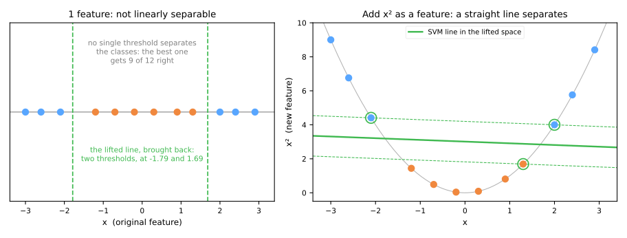
Twelve points on a line cannot be split by one threshold; mapped to (x, x²) a line separates them

Twelve points on a line, the outer ones \(+1\): no threshold on \(x\) beats 0.75.
Add the column \(x^2\) and a plain linear SVM gets 1.00.

The line \(w_1 x + w_2 x^2 + b = 0\) in \((x, x^2)\) becomes two thresholds in \(x\), at −1.79 and 1.69: a linear model in a richer space is a non-linear model in the original one.

The problem is size: with \(d\) features and degree \(p\) there are \(\binom{d+p}{p}\) monomials. With 784 pixels and degree 3: 80,931,145 columns.

The kernel: an inner product without the map

The dual and the prediction touch the data only through inner products:

\[ f(x) = \sum_{i \in \text{SV}} \alpha_i y_i \, \langle x_i, x \rangle + b \qquad\Rightarrow\qquad K(u, v) = \langle \phi(u), \phi(v) \rangle \]

SV: support vectors; \(\alpha_i\): their weights in the dual; \(\phi\): the feature map; \(K\): the kernel.

Through the map

\(\phi(v) = (v_1^2,\ \sqrt2 v_1 v_2,\ v_2^2)\), \(u = (1,2)\), \(v = (3,1)\):

\(\phi(u)\cdot\phi(v) = 9 + 12 + 4 = \mathbf{25}\)

Through the kernel

\(u \cdot v = 5\), so \(K(u,v) = 5^2 = \mathbf{25}\)

A 2-term dot product and a square, however big the map is.

linear	\(u^\top v\)	best for sparse high-dimensional data (text)
polynomial	\((\gamma u^\top v + r)^p\)	\(p\): degree; \(r\) = `coef0` (use 1 to include the lower degrees)
RBF	\(\exp(-\gamma \lVert u - v \rVert^2)\)	the default; infinite-dimensional space; \(\gamma\) sets the reach

RBF is a similarity

Predict. Three points on a line, at 0, 1 and 3. As \(\gamma\) grows, does the similarity between 0 and 3 rise or fall?

\(K(0, 1)\): the RBF kernel between the points at 0 and at 1, \(e^{-\gamma \cdot 1^2}\); \(K(0, 3) = e^{-\gamma \cdot 3^2}\). \(\gamma\) sets how fast similarity fades with distance.

\(\gamma\)	K(0, 1)	K(0, 3)
0.1	0.905	0.407
0.5	0.607	0.011
2	0.135	0.000

\[ f(x) = \sum_{i \in \text{SV}} \alpha_i \, y_i \, e^{-\gamma \lVert x_i - x \rVert^2} + b \]

It is a weighted vote of the support vectors near \(x\). That is k-NN (k nearest neighbors) with two changes: the vote is smooth, and only the support vectors vote, with learned weights. \(\gamma\) plays a role similar to \(1/k\).

Kernels compared

Predict. Circles and moons, 5-fold CV (cross-validation). How much does the linear SVM get on the circles?

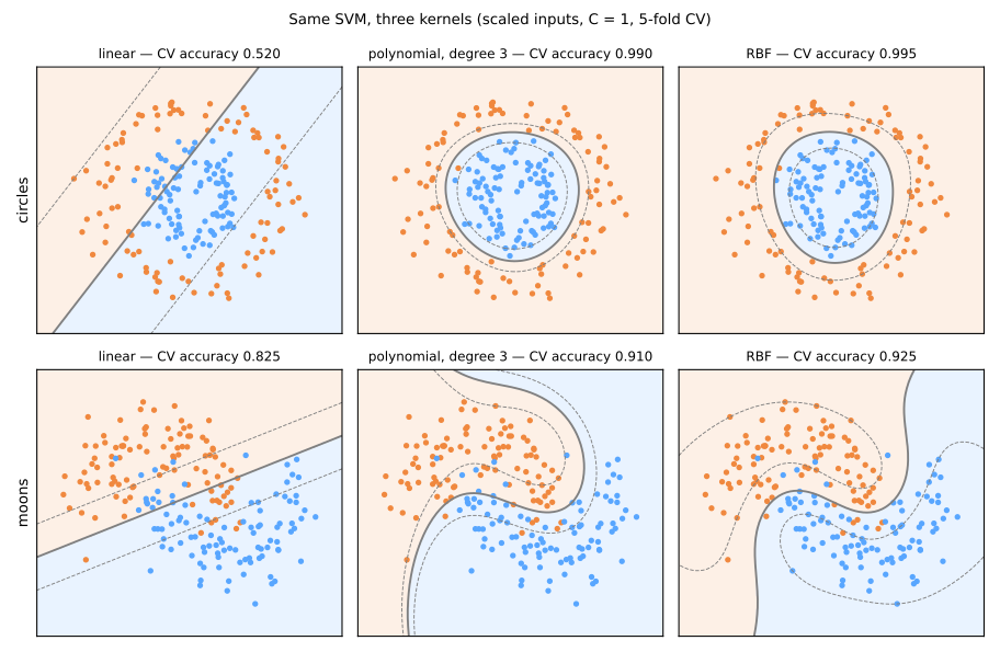
Linear, polynomial and RBF SVMs on circles and moons

	circles	moons
linear	0.520	0.825
poly, degree 3	0.990	0.910
RBF	0.995	0.925

On the circles the linear SVM is at chance. RBF is scikit-learn's default because it rarely does badly; linear is still the right first try when there are many features, as in text.

Stage 2 · How do we set the two knobs?

C and γ together

Predict. \(C\): price of a violation; \(\gamma\): reach of each support vector. Which corner overfits?

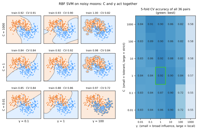
Nine RBF boundaries and the CV accuracy of 36 (C, gamma) pairs

small \(\gamma\): each support vector reaches the whole plane → almost straight boundary, 0.83–0.84 for every \(C\);
large \(\gamma\): each support vector is an island → near-perfect training, CV collapses to 0.55–0.58;
the good diagonal: large \(C\) with small \(\gamma\), or small \(C\) with larger \(\gamma\).

The two knobs trade flexibility for smoothness, so they must be searched together: tuning \(C\) at a fixed, badly chosen \(\gamma\) only finds the best cell of a bad column.

And read the winner with its noise: the between-fold std is 0.022, so "0.920 at \(C = 1, \gamma = 1\)" is a good choice, not a proven optimum.

Scaling is mandatory

Predict. Wine has one feature in the hundreds (proline). What happens to the RBF SVM without a scaler?

	feature stds	no scaler	with scaler
wine	0.124 to 314.0	0.657	0.983
breast cancer	0.003 to 568.9	0.921	0.977

The RBF kernel measures squared Euclidean distance: a feature in the thousands dominates one in fractions, exactly as in k-NN.
gamma='scale' does not fix it: it divides by the variance of all features together, adapting \(\gamma\) to the overall scale, not to the differences between features.

The scaler goes inside the pipeline, so each CV fold fits its own on its own training rows.

Stage 3 · What comes out of the model?

Scores, probabilities and multiclass

Predict. Turning the scores into Platt probabilities: does the ROC AUC go up, down or stay put?

`decision_function` is enough for ROC

the natural output is \(f(x)\): a signed distance in units of the half-margin, \(\pm 1\) at the edges of the street;
not a probability, but it ranks — and ranking is all that ROC AUC (area under the ROC curve) and AP (average precision) need;
ROC AUC from \(f(x)\): 0.9927; from Platt probabilities: 0.9927.

Platt's sigmoid is monotone: it adds calibration, not discrimination. And it costs 5 extra fits.

Multiclass: one-vs-one

SVC trains \(k(k-1)/2\) binary SVMs — 45 for 10 digits — and predicts by majority;
each one sees only the rows of its two digits, about a fifth of the data;
LinearSVC uses one-vs-rest: 10 classifiers.

On digits, standardizing even costs a little (0.987 raw against 0.981): the pixels already share one unit.

Stage 4 · When does it pay off?

When the SVM stops being practical

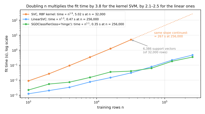
Fit time against n on a log-log scale: kernel SVC grows like n^1.9 while LinearSVC and SGD (stochastic gradient descent) stay almost flat

with \(n\) training rows, fitting costs \(n^2\) to \(n^3\); doubling \(n\) multiplies the time by 3.8;
32,000 rows ≈ 5 s; 256,000 ≈ 4.5 min, for one \((C, \gamma)\) pair; ×125 for a 25-cell grid with 5-fold CV.

`SVC(kernel="linear")`	0.979
`LinearSVC()`	0.955
`SGDClassifier(hinge)`	0.949
`SVC`, one-vs-rest	0.952
`LinearSVC`, one-vs-one	0.979

On digits the gap is one-vs-one against one-vs-rest, not the solver.

Rule of thumb: kernels up to a few tens of thousands of rows. Beyond that, a linear SVM on good features, or models that scale better, like gradient boosting.

Practical profile

	SVM (RBF)	Logistic regression	k-NN
boundary	any smooth shape	linear	any shape, local
what it stores	the support vectors	\(w, b\)	the whole training set
hyperparameters	\(C\) and \(\gamma\), coupled	\(C\)	\(k\), distance
probabilities	no; Platt afterwards	yes, native	vote fractions
training cost	\(\sim n^2\) to \(n^3\)	\(\sim n\)	none
reach for it when	small/medium \(n\), non-linear boundary, many features	you need probabilities or explanations	tiny problems, quick baselines

Advanced lab · about 35 min, in pairs

The kernel and the tuning: steps 5 to 9

Same Colab notebook, from step 5 (Passo 5). New session? Runtime → Run before.
Switching the RBF on with no tuning already takes accuracy from 0.886 to 0.939; tuning \(C\) and \(\gamma\) reaches 0.954.
Simulations: what γ does, seen from inside (step 6) and scaling an already-normalized dataset (step 7).
Steps 8 and 9: tuned rivals on the same folds, and the single test.

Pace: steps 5 and 6 with the simulation in 15 min; step 7 and its simulation in 10 min; steps 8 and 9 in 10 min.