The path of this part
- The widest streetmany lines separate; the margin chooses
- Geometry by handsigned margin, the optimization problem, support vectors
- Soft margin and Cslack, hinge loss, what C buys
Many lines separate — which one?
Predict. The three lines on the left get every training point right. Which one would you trust with a new point?
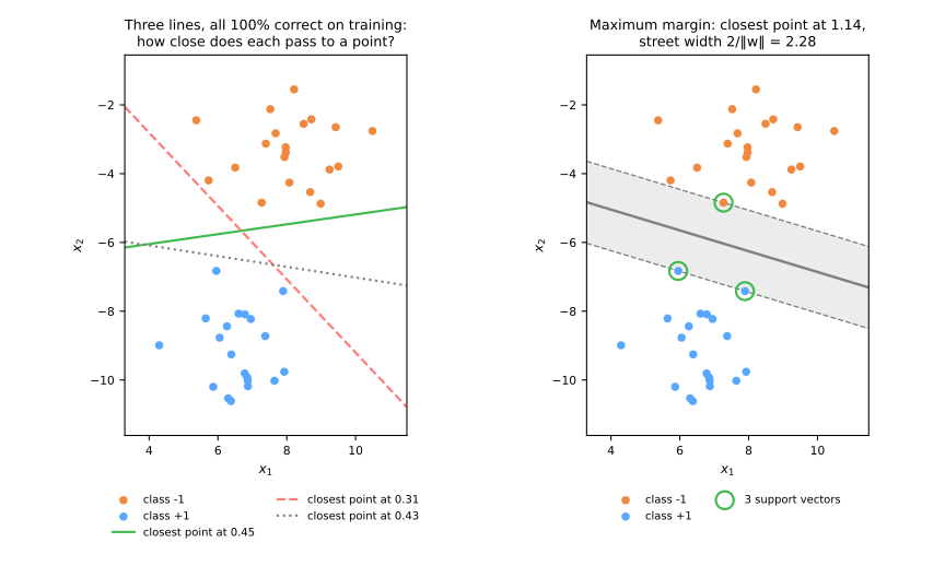
- The three on the left have 100% training accuracy and pass within 0.31–0.45 of some point.
- The max-margin line keeps every point at least 1.14 away; the street is 2.28 wide.
The signed margin
SVMs use \(y \in \{-1, +1\}\), which makes one quantity central:
\[ m = y \cdot f(x), \qquad f(x) = w^\top x + b \]\(x\): a point; \(y\): its label; \(w\): the weight vector, perpendicular to the boundary; \(b\): the intercept. The boundary is \(f(x) = 0\).
\(m > 0\): the point is on the right side; \(m\) large: it is far from the boundary.
And the distance from a point to the hyperplane:
\[ \text{distance}(x) = \frac{\lvert w^\top x + b \rvert}{\lVert w \rVert} \]The optimization problem
\[ \min_{w, b} \; \tfrac{1}{2}\lVert w \rVert^2 \quad \text{subject to} \quad y_i(w^\top x_i + b) \geq 1 \;\; \forall i \]\((x_i, y_i)\): the \(i\)-th training point and its label. The constraint says: every point on its correct side and outside the street.
- maximizing the street \(2/\lVert w \rVert\) is minimizing \(\lVert w \rVert\);
- it is a convex quadratic program: a single global optimum, no random initialization, no learning rate.
Six points, solved by hand
| point | \(x_1\) | \(x_2\) | \(y\) |
|---|---|---|---|
| A | 0 | 0 | −1 |
| B | 1 | 0 | −1 |
| C | 0 | 1 | −1 |
| D | 2 | 2 | +1 |
| E | 3 | 2 | +1 |
| F | 2 | 3 | +1 |
By symmetry, \(w = (a, a)\). The nearest negatives (B, C) sit at \(x_1 + x_2 = 1\); the nearest positive (D) at 4. The boundary goes halfway, at 2.5:
\[ 4a + b = 1,\quad a + b = -1 \;\Rightarrow\; a = \tfrac{2}{3},\; b = -\tfrac{5}{3} \] \[ \lVert w \rVert = 0.943 \quad\Rightarrow\quad \text{street} = 2.121 \]The library agrees: w = [0.667 0.667], b = −1.667, width 2.121, support vectors B, C and D.
Only the support vectors matter
Predict. Delete E and refit; then delete D and refit. Which deletion moves the line?
\[ w = \sum_i \alpha_i \, y_i \, x_i, \qquad \alpha_i = 0 \;\text{ for every point beyond the margin} \]\(\alpha_i \geq 0\): one weight per training point, found by the solver. Here \(\alpha_i y_i = -\tfrac{2}{9}\) for B and C, \(\tfrac{4}{9}\) for D, 0 for A, E and F: \( w = -\tfrac{2}{9}(1, 0) - \tfrac{2}{9}(0, 1) + \tfrac{4}{9}(2, 2) = (\tfrac{2}{3}, \tfrac{2}{3}) \).
| point removed | \(w\) | width |
|---|---|---|
| E = (3, 2) — not a support vector | (0.667, 0.667) | 2.121 (unchanged) |
| D = (2, 2) — is a support vector | (0.5, 0.5) | 2.828 |
Overlapping classes: the soft margin
\[ \min_{w,b,\xi} \; \tfrac{1}{2}\lVert w \rVert^2 + C \sum_i \xi_i \quad \text{with} \quad y_i f(x_i) \geq 1 - \xi_i, \; \xi_i \geq 0 \]\(\xi_i\): the slack, how far point \(i\) is past its edge of the street; \(C\): the price of one unit of slack; \(m_i = y_i f(x_i)\), its signed margin.
The cheapest slack is \(\xi_i = \max(0,\, 1 - m_i)\) — the hinge loss. Substituting:
\[ \min_{w,b} \; \tfrac{1}{2}\lVert w \rVert^2 + C \sum_i \max(0,\, 1 - y_i f(x_i)) \]Hinge against log loss
Predict. Four points of class \(+1\), scored with the six-point solution. Which ones cost nothing under the hinge? And under the log loss?
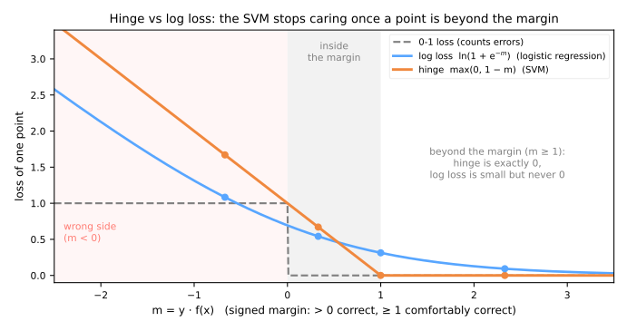
| point | \(m = y f(x)\) | hinge | log loss |
|---|---|---|---|
| (3, 3) | 2.333 | 0.000 | 0.093 |
| (2, 2) | 1.000 | 0.000 | 0.313 |
| (1.5, 1.5) | 0.333 | 0.667 | 0.540 |
| (1, 0.5) | −0.667 | 1.667 | 1.081 |
Both are convex, so they can be optimized with confidence. The hinge is also an upper bound of the 0-1 loss; the log loss, with the natural log, is not quite one: it stays below 1 for \(-0.54 < m \leq 0\).
What C does, measured
| \(C\) | street width | support vectors | train | CV (cross-validation) |
|---|---|---|---|---|
| 0.001 | 9.23 | 78 | 0.99 | 1.000 |
| 0.01 | 5.13 | 27 | 1.00 | 0.990 |
| 0.1 | 2.63 | 12 | 1.00 | 1.000 |
| 1 | 1.33 | 6 | 1.00 | 0.990 |
| 100 | 0.39 | 3 | 1.00 | 0.990 |
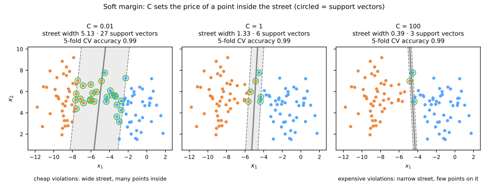
Simulator: what C buys
Predict. Slide \(C\) from small to large. What happens to the street width and to the number of support vectors? Then drag a point far from the street: does the line move?
The linear SVM in five lines
- The margin is the ruler: the street of width \(2/\lVert w \rVert\).
- Maximizing the street = minimizing \(\lVert w \rVert\), with \(y_i f(x_i) \geq 1\). Convex: one global optimum.
- Only the support vectors matter: \(\alpha_i = 0\) beyond the margin.
- The soft margin charges \(C\) per violation; the slack is the hinge loss.
- \(C\) is logistic regression's knob: small = strong regularization = wide street.
| symptom | what to do |
|---|---|
| almost every point is a support vector | raise \(C\) |
| 3 support vectors and training 1.00 | lower \(C\); look at CV |
| the linear boundary does not fit | the kernel, in the advanced part |
Radar: linear models, steps 1 to 4
- Ionosphere: 351 radar returns, 34 features, 64% "good". Small, high-dimensional, non-linear boundary.
- Notebook on Colab (in Portuguese): nothing to download. Save a copy to your Drive.
- In each step, answer the Predict before running.
- Simulations: only the support vectors matter and C changes the width of the street (step 4).
Pace: steps 1 to 3 in 10 min; step 4 and the two simulations in 20 min.