Text Representation
Every technique in the course so far starts from a table of numbers: PCA rotates its columns, k-means measures distances between its rows. Text does not arrive as a table. A customer review, a support ticket, a news post is a string of characters of any length. This lesson builds the bridge from strings to vectors, so that the geometric tools you already know (distances, projections, clusters) apply to text. It is also the groundwork for the next lesson, Topic Modeling & BERTopic, which combines everything here.
There are two families of answers:
- sparse representations (bag-of-words, TF-IDF): one column per word of the vocabulary, a document is its word counts, suitably weighted. Built by counting, in a second, with no model;
- dense representations (word embeddings, sentence embeddings): a few hundred numbers per word or per document, produced by a model trained on large amounts of text, where texts with similar meaning land close together even when they share no words.
Whatever the family, the lesson follows one pipeline in four stages, drawn below: 1. text → tokens; 2. tokens → vector (sparse by counting, dense with a trained model); 3. compare vectors with a similarity or a distance; 4. use and choose, deciding between sparse and dense for search and classification. Stage 2 comes up twice, first for the sparse family and then for the dense one. Each stage links to its section, and in the slides a strip at the bottom shows which stage you are in.
- Text → tokenstokenization, normalization, vocabulary
- Tokens → vectorsparse: bag-of-words, TF-IDF · dense: embeddings
- Compare vectorscosine, Euclidean distance, dot product, Jaccard
- Use and choosesearch and classification: sparse or dense?
This page covers what all of them share (cutting text into tokens, and how the vocabulary grows), gives a map of the four approaches, each with its own page, simulator and lab, prints the vectors each of them produces and the measures used to compare two vectors (cosine, Euclidean distance, dot product), and then measures sparse against dense on the same data, so that you know when to use which. Every number below comes from running the code next to it; each figure is produced by a short Python script that sits next to its page. The toy examples are in Portuguese, so the tokenizer's quirks are the ones you will meet in your own data.
Slides
Click the slides and use the ← → arrows to navigate; F goes full screen and Esc shows every slide. Open the slides in a new tab
Tokenization and the vocabulary
From a string to tokens
Stage 1. The first step is to cut the text into units, tokens, and collect the vocabulary: the set of distinct tokens in the corpus (the collection of documents). Take three short documents:
from sklearn.feature_extraction.text import CountVectorizer

docs = ["O gato comeu o peixe.",                 # the cat ate the fish
        "O cachorro comeu a ração do gato.",     # the dog ate the cat's food
        "Gato dorme, gato sonha."]               # cat sleeps, cat dreams
analyzer = CountVectorizer().build_analyzer()    # scikit-learn's default tokenizer
for d in docs:
    print(analyzer(d))
['gato', 'comeu', 'peixe']
['cachorro', 'comeu', 'ração', 'do', 'gato']
['gato', 'dorme', 'gato', 'sonha']
Three things happened silently, and each is a decision you can change:
- lowercasing: "O" and "o", "Gato" and "gato" are the same token (
lowercase=True); - punctuation is dropped: the default
token_pattern,r"(?u)\b\w\w+\b", keeps runs of two or more letters or digits. Commas and periods vanish; - one-letter words vanish too: the articles "o" and "a" are gone, because they have a single character. In English this mostly removes "a" and "I"; in Portuguese it removes the articles o, a and the conjunction e, but keeps do, da, no, na. Accents are kept ("ração");
strip_accents='unicode'would turn it into "racao".
To see these choices one at a time, take a single sentence and cut it three ways, from the crudest tokenizer to scikit-learn's:
import re

s = "Os gatos não comeram a ração do cachorro, mas o gato comeu!"
# the cats did not eat the dog's food, but the cat ate!
print(s.split())                          # 1. split on whitespace
print(re.findall(r"\w+", s.lower()))      # 2. lowercase, then a word regex
print(analyzer(s))                        # 3. scikit-learn: also drops 1-letter words
['Os', 'gatos', 'não', 'comeram', 'a', 'ração', 'do', 'cachorro,', 'mas', 'o', 'gato', 'comeu!']
['os', 'gatos', 'não', 'comeram', 'a', 'ração', 'do', 'cachorro', 'mas', 'o', 'gato', 'comeu']
['os', 'gatos', 'não', 'comeram', 'ração', 'do', 'cachorro', 'mas', 'gato', 'comeu']
- whitespace split: the cheapest tokenizer. Punctuation sticks to the words, so "cachorro," and "comeu!" would get columns of their own, different from "cachorro" and "comeu"; "Os" and "os" would be two tokens too;
- a word regex:
\w+keeps runs of letters and digits and drops everything else; after lowercasing, the 12 pieces are clean words, including the one-letter "a" and "o"; - scikit-learn's default: the same, minus the one-letter words: 10 tokens.
Stop words, stemming and lemmatization, n-grams
Stop words are the very frequent words that carry little content: the, of, and; de, do, que. scikit-learn ships an English list (stop_words='english') and accepts any list you give it. n-grams are sequences of \(n\) consecutive tokens; ngram_range=(1, 2) keeps single words and pairs of neighbors (bigrams), which buys back a little word order ("não gostei" is not "gostei"):
stop_pt = ['o', 'a', 'os', 'as', 'do', 'da', 'de', 'no', 'na', 'e', 'um', 'uma']   # a tiny stop list
for params in [{}, {'stop_words': stop_pt}, {'ngram_range': (1, 2)}]:
    vocab = CountVectorizer(**params).fit(docs).get_feature_names_out()
    print(params, len(vocab))
    print('   ', list(vocab))
{} 8
    ['cachorro', 'comeu', 'do', 'dorme', 'gato', 'peixe', 'ração', 'sonha']
{'stop_words': ['o', 'a', 'os', 'as', 'do', 'da', 'de', 'no', 'na', 'e', 'um', 'uma']} 7
    ['cachorro', 'comeu', 'dorme', 'gato', 'peixe', 'ração', 'sonha']
{'ngram_range': (1, 2)} 17
    ['cachorro', 'cachorro comeu', 'comeu', 'comeu peixe', 'comeu ração', 'do', 'do gato', 'dorme', 'dorme gato', 'gato', 'gato comeu', 'gato dorme', 'gato sonha', 'peixe', 'ração', 'ração do', 'sonha']
The stop list removed "do": 8 words become 7. Bigrams more than doubled the vocabulary, from 8 columns to 17, on three sentences. Note "comeu peixe": the article between the two words had already been dropped, so the bigram joins words that were not adjacent in the original text.
Two more normalizations reduce the variants of a word to one token. Neither is in scikit-learn; both need a language-specific tool:
| what it does | "sábados" | "comeu", "comeram" | tool | |
|---|---|---|---|---|
| stemming | chops suffixes by rules; the result need not be a word | "sáb" | "com", "com" | NLTK's RSLPStemmer (Portuguese), Porter (English) |
| lemmatization | maps each word to its dictionary form, using a vocabulary and the part of speech | "sábado" | "comeu" (missed), "comer" | spaCy (pt_core_news_sm) |
Both merge columns that mean the same thing ("sábado" and "sábados" will matter in the TF-IDF search engine), at the price of occasionally merging words that do not. With enough data and the dense models of the second half of the lesson, they matter less; for small corpora and keyword search they still help.
The same sentence through each of them (the stop list is the tiny one above):
import nltk      # pip install nltk spacy
import spacy     # python -m spacy download pt_core_news_sm

nltk.download('rslp', quiet=True)                 # the rules of the Portuguese stemmer
stemmer = nltk.stem.RSLPStemmer()
nlp = spacy.load('pt_core_news_sm')               # a small Portuguese model
words = re.findall(r"\w+", s.lower())
print('stop words out:', [w for w in words if w not in stop_pt])
print('stems (RSLP):  ', [stemmer.stem(w) for w in words])
print('lemmas (spaCy):', [t.lemma_ for t in nlp(s) if not t.is_punct])
print('bigrams:       ', CountVectorizer(ngram_range=(2, 2)).build_analyzer()(s))
print('"com" (with) and "comida" (food) stem to:', stemmer.stem('com'), stemmer.stem('comida'))
stop words out: ['gatos', 'não', 'comeram', 'ração', 'cachorro', 'mas', 'gato', 'comeu']
stems (RSLP):   ['os', 'gat', 'não', 'com', 'a', 'raç', 'do', 'cachorr', 'mas', 'o', 'gat', 'com']
lemmas (spaCy): ['o', 'gato', 'não', 'comer', 'o', 'ração', 'de o', 'cachorro', 'mas', 'o', 'gato', 'comeu']
bigrams:        ['os gatos', 'gatos não', 'não comeram', 'comeram ração', 'ração do', 'do cachorro', 'cachorro mas', 'mas gato', 'gato comeu']
"com" (with) and "comida" (food) stem to: com com
Reading each line:
- stop words: the articles and "do" are gone; "não" stays, because it is not in the list. scikit-learn's English list does contain "not", "no" and "never", so
stop_words='english'erases negations: check a stop list before using it; - stemming: "gatos" and "gato" both become "gat", "comeram" and "comeu" both become "com". Neither is a word, and "ração" becomes "raç". The last line shows the price: the preposition "com" (with) and the noun "comida" (food) also become "com", so four unrelated words share one column;
- lemmatization: "gatos" → "gato", "comeram" → "comer", the articles "Os" and "a" → "o", and the contraction "do" is split into "de o". But the small model left "comeu" as it is: a lemmatizer is a statistical model, and it makes mistakes;
- bigrams: nine pairs of neighbors (after scikit-learn's tokenizer), and "não comeram" survives as one feature, the order that a bag of single words loses.
Subwords: the tokenizers of neural models
The dense models of the second half of this lesson do not use a word list at all. Their tokenizers cut text into subwords: frequent words stay whole and rare words are split into frequent pieces, so no word is ever unknown. Here are the tokenizers of the two models used in this lesson, on two English words and on the sentence above:
from transformers import AutoTokenizer           # installed with sentence-transformers

wordpiece = AutoTokenizer.from_pretrained('sentence-transformers/all-MiniLM-L6-v2')
sentpiece = AutoTokenizer.from_pretrained('sentence-transformers/paraphrase-multilingual-MiniLM-L12-v2')
print('vocabularies:', len(wordpiece), 'and', len(sentpiece), 'pieces')
for w in ['tokenization', 'unbelievably']:
    print(f"{w:13s}", wordpiece.tokenize(w))
print('English model:     ', wordpiece.tokenize(s))
print('multilingual model:', sentpiece.tokenize(s))
print('a rare word:       ', sentpiece.tokenize('desparafusaram'))   # they unscrewed
vocabularies: 30522 and 250002 pieces
tokenization  ['token', '##ization']
unbelievably  ['un', '##bel', '##ie', '##va', '##bly']
English model:      ['os', 'ga', '##tos', 'na', '##o', 'come', '##ram', 'a', 'ra', '##cao', 'do', 'ca', '##cho', '##rro', ',', 'mas', 'o', 'ga', '##to', 'come', '##u', '!']
multilingual model: ['▁Os', '▁gato', 's', '▁não', '▁come', 'ram', '▁a', '▁ra', 'ção', '▁do', '▁cachorro', ',', '▁mas', '▁o', '▁gato', '▁come', 'u', '!']
a rare word:        ['▁des', 'para', 'fus', 'aram']
- WordPiece (Schuster & Nakajima, 2012), the tokenizer of BERT and of
all-MiniLM-L6-v2: a vocabulary of 30,522 pieces learned from English text. "tokenization" is "token" + "##ization", where##marks a piece glued to the one before it. On Portuguese it still produces something, but badly: this model lowercases and strips accents ("não" → "na", "##o"; "ração" → "ra", "##cao") and cuts "cachorro" into three meaningless pieces; - SentencePiece (Kudo & Richardson, 2018), the tokenizer of the multilingual model: 250,002 pieces learned from text in 50+ languages;
▁marks the start of a word. Accents and case are kept, frequent words stay whole ("não", "cachorro") and inflections are split off: "gatos" → "gato" + "s", "comeram" → "come" + "ram"; - a rare word such as "desparafusaram" (they unscrewed) becomes four known pieces. Each piece has its own vector inside the model, so a word never seen as a whole still gets a representation. This is the "handled (subword pieces)" row of the comparison table at the end of the page; a sparse vocabulary would simply have no column for it.
Where each of these decisions applies. Lowercasing, stop words, stemming and n-grams are decisions of the sparse family, because they define the columns. In the dense models the tokenizer and the vocabulary come with the model, and the text goes in as it is:
| bag-of-words, TF-IDF | word embeddings (GloVe) | sentence embeddings | |
|---|---|---|---|
| lowercase, punctuation | your choice (scikit-learn's default lowercases and drops punctuation) | GloVe's vocabulary is all lowercase | the model's tokenizer decides |
| stop words | optional: removes columns | optional, before averaging | no: "não" changes the meaning |
| stemming, lemmatization | optional: merges columns | no: one vector per form ("cat", "cats") | no |
| n-grams | optional: columns for pairs | no | no: the model reads the sentence in order |
| subwords | no | no: a word outside the vocabulary gets no vector | yes, the model's tokenizer |
How big does the vocabulary get?
Three sentences gave 8 words. A real corpus: the 20 Newsgroups collection (Lang, 1995), about 18,000 posts from 20 Usenet discussion groups of the early 1990s, shipped with scikit-learn. We use the 11,314 posts of its training part, with headers, signatures and quoted replies removed, read them one token at a time and count how many distinct words we have seen so far:
import numpy as np
from sklearn.datasets import fetch_20newsgroups

news = fetch_20newsgroups(subset='train', remove=('headers', 'footers', 'quotes'))
seen, n_tokens, curve = set(), 0, []
for post in news.data:
    for tok in analyzer(post):
        n_tokens += 1
        seen.add(tok)
    curve.append((n_tokens, len(seen)))        # (N tokens read, V distinct words) after each post
curve = np.array(curve, dtype=float)

fit = curve[:, 0] > 1000
beta, logK = np.polyfit(np.log(curve[fit, 0]), np.log(curve[fit, 1]), 1)
print(f"{len(news.data):,} posts · {n_tokens:,} tokens · {len(seen):,} distinct words")
print(f"Heaps fit: V = {np.exp(logK):.1f} · N^{beta:.2f}")
for N in [10_000, 100_000, 1_000_000]:
    i = np.searchsorted(curve[:, 0], N)
    print(f"after {curve[i, 0]:>9,.0f} tokens: {curve[i, 1]:>7,.0f} words   (fit: {np.exp(logK) * curve[i, 0] ** beta:>7,.0f})")
11,314 posts · 2,158,589 tokens · 101,631 distinct words
Heaps fit: V = 15.0 · N^0.61
after    11,025 tokens:   3,279 words   (fit:   4,246)
after   100,504 tokens:  18,692 words   (fit:  16,210)
after 1,000,517 tokens:  63,306 words   (fit:  65,283)
Two empirical laws show up in these numbers, one per figure.
Heaps' law (Heaps, 1978): the vocabulary grows like a power of the text length, \(V \approx K N^{\beta}\), with \(\beta\) between 0.4 and 0.7 in most corpora.
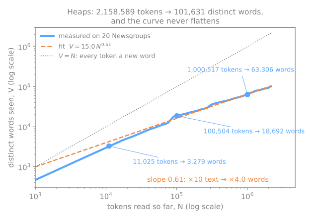
How to read it: the x axis is the number of tokens read so far and the y axis the number of distinct words seen; both are on a log scale, where a power law becomes a straight line whose slope is the exponent. The dotted line is what the curve would look like if every token were a new word. Here \(\beta = 0.61\): ten times more text gives about \(10^{0.61} \approx 4\) times more words (11 thousand tokens give 3,279 words, 100 thousand give 18,692, a million give 63,306). It never levels off, because new names, typos, numbers and jargon keep arriving. A vocabulary built today will meet words it has never seen tomorrow, and a sparse representation has no column for them.
Zipf's law (Zipf, 1949): frequency falls roughly as a power of rank.
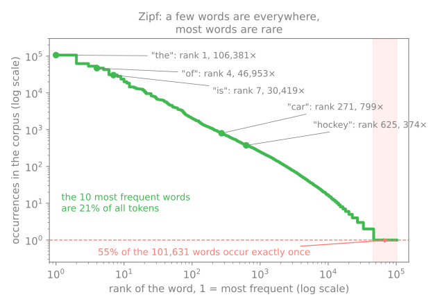
How to read it: each point is a word, placed by its rank (1 = most frequent) on the x axis and by how many times it occurs on the y axis, both on a log scale. At the top, "the" occurs 106,381 times and the 10 most frequent words make up 21% of all tokens; in the middle, "car" (rank 271) occurs 799 times; in the red band, 55% of the 101,631 words appear exactly once. Most columns of a bag-of-words matrix describe a single document, and the few words at the top are precisely the stop words.
Both laws already show up in one paragraph. Edit the text below and switch the tokenization choices one at a time: lowercase, punctuation, stop words, unigrams or bigrams. Watch the vocabulary size \(V\), the share of terms that appear only once and the small Heaps curve on the right. The simulator cuts words like the word regex above, so one-letter words are kept and the stop list has something to remove.
Every choice changes \(V\): keeping case or punctuation adds columns, removing stop words takes away the most frequent ones. Even in a hundred words most terms appear once, and with bigrams the curve almost follows the diagonal, because nearly every pair of neighbors is new.
A map of the approaches
Stage 2. Once the text is cut into tokens, the four pages of this lesson turn those tokens into vectors in four different ways, from the simplest to the most powerful:
| page | a document becomes | built from | what it cannot do |
|---|---|---|---|
| U4.1 Bag-of-words | its word counts, one column per word | counting, no model | see word order, synonyms, or words not seen in fit |
| U4.2 TF-IDF | counts weighted by how rare each word is | counting over the corpus | the same: it only reweights the columns |
| U4.3 Word embeddings | a dense vector per word (average them for a document) | co-occurrence in a large corpus | tell apart the senses of one word |
| U4.4 Sentence embeddings | one dense vector per sentence or short document | a pretrained transformer | be cheap, or explain its dimensions |
Bag-of-Words
The simplest representation: a document becomes the vector of its word counts, one column per vocabulary word, and the order of the words is thrown away. The three documents above become a 3 × 8 matrix:
import pandas as pd

bow = CountVectorizer()
X = bow.fit_transform(docs)                        # sparse matrix: 3 rows, 8 columns
print(pd.DataFrame(X.toarray(), columns=bow.get_feature_names_out(), index=['doc 1', 'doc 2', 'doc 3']))
       cachorro  comeu  do  dorme  gato  peixe  ração  sonha
doc 1         0      1   0      0     1      1      0      0
doc 2         1      1   1      0     1      0      1      0
doc 3         0      0   0      1     2      0      0      1
Each row is a document, each column a word, each cell a count: "gato" appears twice in document 3 ("Gato dorme, gato sonha"). Of the 24 cells, 13 are already zero. The 11,314 newsgroup posts become a 11,314 × 101,631 matrix that is 99.90% zeros, stored in a sparse format that keeps only the non-zero cells. Raw counts are led by function words ("the" is in 9,475 of the 11,314 posts), which is why they are rarely used unweighted. The bag-of-words page builds the matrix by hand and with CountVectorizer, compares counts with presence (binary=True), measures the cost of n-grams, and has a simulator and a lab.
TF-IDF
TF-IDF (term frequency × inverse document frequency) multiplies each count by a weight that falls with the number of documents containing the word. scikit-learn's version, for a word \(t\) in a document \(d\) of a corpus of \(n\) documents, \(\text{df}(t)\) of which contain \(t\):
followed by dividing each row by its length. On the three documents above:
from sklearn.feature_extraction.text import TfidfVectorizer

tfidf = TfidfVectorizer()
T = tfidf.fit_transform(docs)
print(pd.DataFrame([tfidf.idf_], columns=tfidf.get_feature_names_out(), index=['idf']).round(4))
print(pd.DataFrame(T.toarray(), columns=tfidf.get_feature_names_out(), index=['doc 1', 'doc 2', 'doc 3']).round(3))
     cachorro   comeu      do   dorme  gato   peixe   ração   sonha
idf    1.6931  1.2877  1.6931  1.6931   1.0  1.6931  1.6931  1.6931
       cachorro  comeu     do  dorme   gato  peixe  ração  sonha
doc 1     0.000  0.548  0.000  0.000  0.425   0.72  0.000  0.000
doc 2     0.505  0.384  0.505  0.000  0.298   0.00  0.505  0.000
doc 3     0.000  0.000  0.000  0.543  0.641   0.00  0.000  0.543
"gato", present in all three documents, gets idf 1, "comeu", in two, gets 1.2877, and a word present in only one gets 1.6931. Compare document 1 with its row in the bag-of-words: the counts were 1, 1, 1; now "gato" weighs 0.425 and "peixe", which only document 1 has, 0.720. Each row has length 1, and the zeros are where they were. The idea goes back to Spärck Jones (1972) and became the standard of information retrieval with Salton & Buckley (1988). The TF-IDF page computes every number by hand, checks that TfidfVectorizer agrees to the fourth decimal, compares documents with the cosine similarity, and builds a small search engine.
Similarity and distance
Stage 3. Once two texts are vectors, "how alike are they?" becomes a number computed from the two vectors. Four measures cover almost every use:
- cosine similarity: compares the directions of the two vectors and ignores their lengths. 1 means they point the same way (the same words in the same proportions), 0 means they share nothing; with counts it is never negative. It is the measure used everywhere in this lesson;
- Euclidean distance: the straight-line distance between the two points, the one k-means uses. 0 means identical vectors; it grows with every difference, including a difference in length;
- dot product: multiply the two vectors coordinate by coordinate and add. Large when both have large values in the same columns, so it grows with the length of the documents;
- Jaccard similarity: forget the counts and compare the two sets of tokens: the number of shared tokens divided by the number of distinct tokens in either. 1 means the same set of words, 0 no word in common.
Take document 1 of the bag-of-words, document 3, and a third document that is document 1 written three times, the same content, three times longer:
from sklearn.metrics import jaccard_score
from sklearn.metrics.pairwise import cosine_similarity, euclidean_distances

A, B, A3 = bow.transform(["O gato comeu o peixe.",
                          "Gato dorme, gato sonha.",
                          "O gato comeu o peixe. " * 3]).toarray()    # A3: document A three times
print('columns:', list(bow.get_feature_names_out()))
print('A  =', A, ' B =', B, ' A3 =', A3)
for name, u, v in [('A and B ', A, B), ('A and A3', A, A3), ('B and A3', B, A3)]:
    print(f"{name}  cosine {cosine_similarity([u], [v])[0, 0]:.3f} · Euclidean {euclidean_distances([u], [v])[0, 0]:.3f}"
          f" · dot {u @ v:2d} · Jaccard {jaccard_score(u > 0, v > 0):.3f}")
columns: ['cachorro', 'comeu', 'do', 'dorme', 'gato', 'peixe', 'ração', 'sonha']
A  = [0 1 0 0 1 1 0 0]  B = [0 0 0 1 2 0 0 1]  A3 = [0 3 0 0 3 3 0 0]
A and B   cosine 0.471 · Euclidean 2.236 · dot  2 · Jaccard 0.200
A and A3  cosine 1.000 · Euclidean 3.464 · dot  9 · Jaccard 1.000
B and A3  cosine 0.471 · Euclidean 4.583 · dot  6 · Jaccard 0.200
Read it as a search problem: the query is A, and the candidates are B (a different subject that shares only "gato") and A3 (exactly the same subject, only longer).
- cosine says what we want: A3 is identical to A (1.000) and B is a partial match (0.471). And B against A3 gets the same 0.471 as B against A: repeating a document does not change its direction;
- Euclidean distance gets it backwards: A3 is farther from A (3.464) than B is (2.236), only because A3 is longer;
- dot product grows with length: B against A3 scores 6, three times its score against A, for the same content;
- Jaccard agrees with cosine here (1.000 and 0.200) because it only looks at which words are present, which also makes it blind to how often they appear.
That is why the cosine is the default for text: documents have every length, and the length of a document says little about its subject. When the vectors are first scaled to length 1, the three measures agree: the dot product is the cosine, and the Euclidean distance ranks every pair in the opposite order of the cosine. TF-IDF rows already have length 1 (scikit-learn divides each row by its length), and sentence embeddings are usually requested with normalize_embeddings=True, so in practice they are compared by a dot product.
The limits of sparse representations
In bag-of-words and TF-IDF, every word is its own axis, orthogonal to all the others. The TF-IDF page measures the consequences on pairs of sentences:
- synonyms score zero: "o carro é rápido" and "o automóvel é veloz" (the car is fast / the automobile is quick) have cosine 0.00;
- word order is invisible: "the dog bit the man" and "the man bit the dog" have cosine 1.00;
- one spelling, two meanings: manga (sleeve or mango) makes two unrelated sentences look alike, while two sentences with the same meaning and different words look unrelated (0.14 in both cases);
- new words vanish: a word not seen during
fithas no column, and a sentence made only of new words becomes the zero vector.
In the TF-IDF lab, the 10 best results for "image" and the 10 best for "picture" have no post in common. These are the failures that motivated dense representations.
Dense embeddings
Back to stage 2, now for the dense family.
"You shall know a word by the company it keeps" (Firth, 1957). The distributional hypothesis (Harris, 1954) says that words used in similar contexts have similar meanings: "car" and "automobile" rarely occur in the same sentence, but they occur next to the same words (engine, dealer, tires). Dense representations exploit this. Instead of one column per word, every word or text gets a vector of a few hundred numbers, learned from a large corpus so that similar contexts give nearby vectors. No single number means anything on its own; only distances between vectors do.
Word embeddings
word2vec (Mikolov et al., 2013) learns one vector per word by training a small network to predict the words around each word; GloVe (Pennington et al., 2014) reaches similar vectors by factorizing a table of co-occurrence counts. Synonyms end up close, and some directions of the space encode relations. The limitation is one vector per word, whatever its sense. The word embeddings page covers how these vectors are learned and what they capture.
What one of these vectors looks like: the pretrained GloVe vectors, trained on 6 billion tokens of English news and Wikipedia, in their smallest version (400,000 words, 50 numbers each). They are English vectors, so the examples are English words:
import gensim.downloader as api                   # pip install gensim

glove = api.load('glove-wiki-gigaword-50')        # ~66 MB, downloaded once
print('cat =', glove['cat'][:8].round(3), '... (50 numbers, none of them zero)')
print('nearest to cat:', ', '.join(f"{w} {c:.2f}" for w, c in glove.most_similar('cat', topn=5)))
for a, b in [('car', 'automobile'), ('car', 'banana')]:
    print(f"cosine {a} / {b}: {glove.similarity(a, b):.2f}")
cat = [ 0.453 -0.501 -0.537 -0.016  0.222  0.546 -0.673 -0.689] ... (50 numbers, none of them zero)
nearest to cat: dog 0.92, rabbit 0.85, monkey 0.80, rat 0.79, cats 0.79
cosine car / automobile: 0.70
cosine car / banana: 0.22
The 50 numbers of "cat" mean nothing one by one; what carries the meaning is which vectors are nearby, measured by the cosine: the nearest words to "cat" are other animals, led by "dog" (0.92). "car" and "automobile", which never shared a column in the bag-of-words, now have cosine 0.70, against 0.22 for "car" and "banana".
Sentence embeddings: contextual and whole-document
Transformer models such as BERT (Devlin et al., 2019) compute the vector of each token from the whole sentence around it, so manga gets a different vector next to "camisa" than next to "madura". Sentence-BERT (Reimers & Gurevych, 2019) trains such a model so that one vector summarizes a whole sentence or short document, and the cosine between two of these vectors tracks how close their meanings are. The sentence-transformers library packages hundreds of such models, several of them multilingual. The sentence embeddings page covers how they are built and how to use them; the rest of this page uses one of them.
It is a small multilingual model from sentence-transformers (the sentence embeddings page explains it): each text becomes 384 numbers, and texts in 50+ languages share the same space. Loading it downloads about 470 MB the first time.
# pip install sentence-transformers
from sentence_transformers import SentenceTransformer

model = SentenceTransformer('paraphrase-multilingual-MiniLM-L12-v2')
emb = model.encode(["o carro é rápido",          # the car is fast
                    "o automóvel é veloz",       # the automobile is quick: same meaning, no shared word
                    "a taxa de juros subiu"],    # the interest rate went up: unrelated
                   normalize_embeddings=True)
print(emb.shape)
print('o carro é rápido =', emb[0][:8].round(3), '... (384 numbers)')
for j in [1, 2]:
    print(f"vs {j}: cosine {cosine_similarity(emb[[0]], emb[[j]])[0, 0]:.2f} · dot {emb[0] @ emb[j]:.2f}"
          f" · Euclidean {euclidean_distances(emb[[0]], emb[[j]])[0, 0]:.2f}")
(3, 384)
o carro é rápido = [ 0.016  0.033 -0.08   0.037 -0.014 -0.002  0.039 -0.028] ... (384 numbers)
vs 1: cosine 0.97 · dot 0.97 · Euclidean 0.25
vs 2: cosine 0.23 · dot 0.23 · Euclidean 1.24
A whole sentence is now 384 numbers, whatever its length. The paraphrase, with no word in common, gets cosine 0.97; the unrelated sentence 0.23. Because the vectors were scaled to length 1 (normalize_embeddings=True), the dot product equals the cosine and the Euclidean distance tells the same story in reverse: small for the paraphrase, large for the unrelated pair.
Sparse vs dense representations
The two families produce vectors of very different shapes. Take one English sentence, so that all three can read it, and represent it three ways: a bag-of-words over the vocabulary of the 11,314 newsgroup posts, the average of its GloVe word vectors, and the sentence embedding:
import numpy as np

s_en = "the cat sleeps on the couch"
bow_news = CountVectorizer().fit(news.data)                  # the 101,631 words of the newsgroups
x = bow_news.transform([s_en])
vocab = bow_news.get_feature_names_out()
print(f"bag-of-words   length {x.shape[1]:>7,} · non-zero {x.nnz:>3}:",
      ', '.join(f"{vocab[j]} (column {j:,}) = {v}" for j, v in zip(x.indices, x.data)), '· all others 0')
g = np.mean([glove[w] for w in s_en.split()], axis=0)        # average of the 6 word vectors
print(f"GloVe average  length {g.size:>7,} · non-zero {np.count_nonzero(g):>3}:", g[:6].round(3), '...')
e = model.encode(s_en)
print(f"sentence emb.  length {e.size:>7,} · non-zero {np.count_nonzero(e):>3}:", e[:6].round(3), '...')
bag-of-words   length 101,631 · non-zero   5: cat (column 26,019) = 1, couch (column 30,064) = 1, on (column 68,080) = 1, sleeps (column 83,252) = 1, the (column 88,532) = 2 · all others 0
GloVe average  length      50 · non-zero  50: [ 0.271  0.037 -0.335 -0.147  0.541  0.055] ...
sentence emb.  length     384 · non-zero 384: [ 0.39  -0.348 -0.135  0.145  0.115  0.278] ...
| sparse (bag-of-words, TF-IDF) | dense (word and sentence embeddings) | |
|---|---|---|
| length | one column per vocabulary word: here 101,631 | fixed by the model: 50 for this GloVe, 384 for this sentence model |
| non-zero values | only the words of the text: here 5 | all of them |
| what one coordinate means | readable: column 26,019 is "how many times cat appears" | nothing on its own; only distances between vectors mean something |
| how it is stored | only the non-zero cells (index, value) | a plain array of floats |
| two texts with no word in common | no shared non-zero column: cosine 0 | can still be close |
Sparse means almost every coordinate is zero, and the few non-zero ones are readable: each is a word of the text. Dense means every coordinate has a value, none readable alone, and the information lives in the geometry. That is the whole difference between the two halves of this lesson, and it decides everything that follows: sparse vectors can only match texts that share words; dense vectors can match texts that share meaning.
Now compare the four techniques yourself. Pick two sentences, or one of the preset pairs, and look at the two vectors under each representation, the bag-of-words and TF-IDF strips almost empty, the dense ones full, and at the cosine, the Euclidean distance and the dot product under each. Start with the paraphrase (no word in common), then the word order, then the ambiguous word bank (a bank that raises interest rates, the bank of a river) against the pair with the same meaning in other words; finally tick B three times and unit length and watch which numbers move. GloVe vectors exist only for English, so with the Portuguese sentences that band averages the English sentence of the same item.
On the paraphrase, the two sparse representations give cosine 0 and the two dense ones do not. With the word order swapped, bag-of-words, TF-IDF and the GloVe average are identical, since none of them sees order, and only the sentence embedding moves a little. Repeating B changes the Euclidean distance and the dot product of the bag-of-words, but not its cosine; at unit length, the dot product and the cosine become the same number.
Sparse vs dense: when to use which
Stage 4. Everything in this section is measured with the multilingual model loaded above, against TF-IDF from scikit-learn.
Similarity: the same pairs, both ways
The pairs of the limits section, and a few more. The TF-IDF is fitted on all the sentences of the table:
pairs_all = [("o carro é rápido", "o automóvel é veloz"),
             ("comprei um celular novo", "adquiri um smartphone novo"),
             ("o gato dorme no sofá", "the cat sleeps on the couch"),
             ("a manga da camisa rasgou", "o punho da blusa descosturou"),
             ("a manga da camisa rasgou", "comi uma manga madura"),
             ("o filme é muito bom", "o filme não é bom"),
             ("o cachorro mordeu o homem", "o homem mordeu o cachorro"),
             ("a taxa de juros subiu", "o time venceu o jogo")]
sentences = list(dict.fromkeys(s for p in pairs_all for s in p))   # unique, in order
tf_pairs = TfidfVectorizer().fit(sentences)
rows = []
for a, b in pairs_all:
    e = model.encode([a, b], normalize_embeddings=True)
    rows.append({'A': a, 'B': b,
                 'TF-IDF': cosine_similarity(tf_pairs.transform([a, b]))[0, 1],
                 'embedding': e[0] @ e[1]})
print(pd.DataFrame(rows).round(2).to_string(index=False))
                        A                            B  TF-IDF  embedding
         o carro é rápido          o automóvel é veloz    0.00       0.97
  comprei um celular novo   adquiri um smartphone novo    0.43       0.91
     o gato dorme no sofá  the cat sleeps on the couch    0.00       0.98
 a manga da camisa rasgou o punho da blusa descosturou    0.21       0.87
 a manga da camisa rasgou        comi uma manga madura    0.21       0.35
      o filme é muito bom            o filme não é bom    0.60       0.46
o cachorro mordeu o homem    o homem mordeu o cachorro    1.00       0.98
    a taxa de juros subiu         o time venceu o jogo    0.00       0.14
Row by row:
- paraphrases ("I bought a new phone" / "I purchased a new smartphone"): 0.91 against 0.43; TF-IDF only sees "um" and "novo";
- translation (row 3): the Portuguese sentence and its English translation share no token, and the multilingual model puts them at 0.98. A query in Portuguese can retrieve documents written in English;
- the two "manga" rows: TF-IDF gives both pairs the same 0.21, while the embedding separates the sleeve-and-cuff pair (0.87) from the sleeve-and-mango pair (0.35);
- negation ("the film is very good" / "the film is not good"): the embedding is lower than TF-IDF (0.46 against 0.60), but far from "opposite". Two sentences about how good the same film is overlap a lot in meaning;
- word order: 0.98. Sentence embeddings blur who bit whom too;
- unrelated sentences score 0.14, not 0. Embedding cosines live on a compressed scale: the ranking (0.97 against 0.14) carries the information, not the absolute value, and a threshold tuned for one model does not transfer to another.
Exact rare tokens: where TF-IDF is stronger
Two help-desk entries that differ only in an error code, and a query for each code:
entries = ["O que fazer quando aparece o erro 0x80070005 na instalação?",
           "O que fazer quando aparece o erro 0x80004005 na atualização?"]
tf_entries = TfidfVectorizer().fit(entries)
E_entries = model.encode(entries, normalize_embeddings=True)
for q in ["erro 0x80070005", "erro 0x80004005"]:
    t = cosine_similarity(tf_entries.transform([q]), tf_entries.transform(entries))[0]
    e = E_entries @ model.encode(q, normalize_embeddings=True)
    print(f"{q}:  TF-IDF {t.round(2)}   embedding {e.round(2)}")
erro 0x80070005:  TF-IDF [0.55 0.18]   embedding [0.8  0.77]
erro 0x80004005:  TF-IDF [0.18 0.55]   embedding [0.81 0.78]
Both representations put the right entry first, but look at the margins. For TF-IDF the code is the most distinctive token of each entry and decides the match, 0.55 against 0.18. For the embedding, both entries are "an error message during installation or update", and the code moves the score by only 0.03 (0.80 against 0.77). With hundreds of similar codes, product names or legal references, exact matching is what you want; production search systems often combine both rankings (hybrid search).
Classification: how many labels do you have?
Most projects eventually need a prediction (route a ticket, tag a post), and the representation becomes the input of a supervised model. None has been taught yet, so we use a logistic regression as a black box (it has its own lesson later): it receives a vector and a label for each training post and learns to predict the labels of new posts. Only the representation changes.
Four newsgroups of the 20 Newsgroups collection (cars, medicine, space, guns), with scikit-learn's official split: the model learns from older posts and is scored on later ones, a hold-out it never sees during training. To see how much labeled data each representation needs, we train with 5, 10, 25 and 100 labeled posts per class, then with all of them:
from sklearn.datasets import fetch_20newsgroups
from sklearn.linear_model import LogisticRegression

def load(subset, cats):
    d = fetch_20newsgroups(subset=subset, categories=cats,
                           remove=('headers', 'footers', 'quotes'), random_state=0)
    keep = [i for i, t in enumerate(d.data) if len(t.split()) >= 20]   # drop empty/very short posts
    return [d.data[i] for i in keep], d.target[keep]

cats = ['rec.autos', 'sci.med', 'sci.space', 'talk.politics.guns']
docs_tr, y_tr = load('train', cats)       # older posts
docs_te, y_te = load('test', cats)        # later posts: the hold-out
E_tr = model.encode(docs_tr, normalize_embeddings=True)
E_te = model.encode(docs_te, normalize_embeddings=True)
print(len(docs_tr), 'training posts ·', len(docs_te), 'test posts')

rng = np.random.default_rng(0)
print('labeled posts per class | TF-IDF + clf | embedding + clf')
for n in [5, 10, 25, 100, 'all']:
    if n == 'all':
        idx = np.arange(len(docs_tr))
    else:
        idx = np.concatenate([rng.choice(np.flatnonzero(y_tr == c), n, replace=False) for c in range(4)])
    vec = TfidfVectorizer(stop_words='english').fit([docs_tr[i] for i in idx])
    sparse_clf = LogisticRegression(max_iter=2000).fit(vec.transform([docs_tr[i] for i in idx]), y_tr[idx])
    dense_clf = LogisticRegression(max_iter=2000).fit(E_tr[idx], y_tr[idx])
    print(f"{str(n):>23s} | {sparse_clf.score(vec.transform(docs_te), y_te):11.3f} | "
          f"{dense_clf.score(E_te, y_te):15.3f}")
2097 training posts · 1364 test posts
labeled posts per class | TF-IDF + clf | embedding + clf
                      5 |       0.557 |           0.819
                     10 |       0.601 |           0.851
                     25 |       0.725 |           0.886
                    100 |       0.850 |           0.897
                    all |       0.904 |           0.901
The score is accuracy on the 1,364 test posts; always guessing one class would get about 25%. With 5 labeled posts per class, the classifier on embeddings reaches 81.9% and the one on TF-IDF 55.7%. With 20 training posts in total, TF-IDF has seen only a few hundred distinct words, and a test post that happens to use none of them is a zero vector. The embedding model arrives already knowing that "sedan" is near "car", from the text it was trained on. As labels accumulate, TF-IDF learns the vocabulary of each class from the data itself, and with all 2,097 posts the two are tied: 90.4% against 90.1%.
What the scores do not show is cost. On the laptop used to write this page, TfidfVectorizer processes the 2,097 training posts in 0.2 seconds, while the embedding model needs about a minute on the same CPU (10 seconds on the laptop's GPU), after a 470 MB download.
| Sparse (bag-of-words, TF-IDF) | Dense (sentence embeddings) | |
|---|---|---|
| size of a document vector | \(\lvert V \rvert\) columns (10⁴–10⁶), 99.9% zeros | 384–1,024 numbers, all non-zero |
| synonyms, paraphrases | orthogonal: cosine 0.00 | nearby: cosine 0.97 |
words never seen in fit | dropped | handled (subword pieces) |
| rare exact tokens (codes, names, jargon) | high idf, strong signal | blurred into the general meaning |
| other languages | separate vocabularies | shared space with a multilingual model |
| few labeled examples (5 per class, above) | 55.7% | 81.9% |
| many labeled examples (all 2,097, above) | 90.4% | 90.1% |
| interpretability | each column is a word | columns are abstract |
| cost | fractions of a second on a CPU, no model | a pretrained model; a GPU helps |
| typical uses | keyword search, strong linear baselines, domain jargon | semantic search, few labels, clustering, BERTopic |
In practice: start with TF-IDF, which is cheap and hard to beat when labeled data and domain vocabulary are plentiful; reach for embeddings when meaning matters more than exact words (search, short texts, paraphrases, several languages) or when labels are scarce; and when both exact tokens and meaning matter, combine them.
Where this leads
Topic Modeling & BERTopic uses both halves of this lesson. It embeds documents with a sentence-transformer, reduces the vectors with UMAP, groups them with HDBSCAN, and then describes each group with a variant of TF-IDF computed per cluster. That pipeline is BERTopic.
Exercises
- With the Heaps fit of this page (\(V = 15.0\,N^{0.61}\)), how many distinct words would you expect in a corpus ten times larger (about 21.6 million tokens)? What does this imply for a vocabulary fitted today and used for a year?
- Tokenize "Não gostei do filme, não!" with scikit-learn's default analyzer, with the tiny stop list of this page, and with
ngram_range=(1, 2). Which version keeps the negation? - For each task, choose sparse or dense and justify in one sentence: (a) find the contract that cites "Lei 13.709/2018"; (b) group 50,000 customer reviews by subject; (c) classify 300 support tickets into 5 queues, with 20 labeled examples; (d) search English papers with Portuguese queries.
Lab: sparse vs dense on real posts
Four newsgroups of the 20 Newsgroups collection (computer graphics, baseball, electronics and Christianity), about 2,100 posts, represented twice: with TF-IDF and with sentence embeddings. The lab puts the two side by side on the tasks of this page: finding posts about the same subject, answering search queries, drawing a map, and feeding a black-box classifier with many and with few labels. The bag-of-words and TF-IDF labs look inside the sparse representation of the same posts.
The lab runs in about two minutes on a CPU; step 2, which encodes every post with a neural network, is most of it (a Colab GPU runtime makes it a few seconds). Run the blocks in order, in one session. To work on it directly, download the lab notebook and open it in Jupyter or Colab (File → Upload notebook).
Step 1 — load the posts
# In Colab, run once:  !pip install sentence-transformers
import numpy as np
import pandas as pd
from sklearn.datasets import fetch_20newsgroups

cats = ['comp.graphics', 'rec.sport.baseball', 'sci.electronics', 'soc.religion.christian']
raw = fetch_20newsgroups(subset='train', categories=cats,
                         remove=('headers', 'footers', 'quotes'), random_state=0)
keep = [i for i, t in enumerate(raw.data) if len(t.split()) >= 20]   # drop empty/very short posts
docs = [raw.data[i] for i in keep]
y = raw.target[keep]
names = np.array(raw.target_names)
print(len(docs), 'posts:', ', '.join(f"{g} {c}" for g, c in zip(names, np.bincount(y))))
print(f"words per post: median {np.median([len(d.split()) for d in docs]):.0f}")
2116 posts: comp.graphics 521, rec.sport.baseball 495, sci.electronics 535, soc.religion.christian 565
words per post: median 97
The same 2,116 posts as in the bag-of-words and TF-IDF labs: four balanced groups, with headers, signatures and quoted replies removed and posts shorter than 20 words dropped. A median post has 97 words.
Step 2 — two representations of the same posts
from sentence_transformers import SentenceTransformer
from sklearn.feature_extraction.text import TfidfVectorizer

tfidf = TfidfVectorizer(stop_words='english', min_df=2)
T = tfidf.fit_transform(docs)
sparse_mb = (T.data.nbytes + T.indices.nbytes + T.indptr.nbytes) / 1e6
print(f"TF-IDF:     {T.shape}, {T.nnz / T.shape[0]:.0f} non-zeros per post, {sparse_mb:.1f} MB")

model = SentenceTransformer('all-MiniLM-L6-v2')      # English, 384 dimensions, ~90 MB
E = model.encode(docs, batch_size=64, normalize_embeddings=True)
print(f"embeddings: {E.shape}, all non-zero, {E.nbytes / 1e6:.1f} MB · reads at most {model.max_seq_length} tokens per post")
TF-IDF:     (2116, 12001), 58 non-zeros per post, 1.5 MB
embeddings: (2116, 384), all non-zero, 3.3 MB · reads at most 256 tokens per post
How to read it:
- TF-IDF: 12,001 columns, but a post fills only 58 of them on average; stored sparse, the whole matrix takes 1.5 MB.
- Embeddings: 384 columns, all non-zero, 3.3 MB in 32-bit floats. Fewer columns, but more memory than the sparse matrix here, because nothing is zero.
- 256 tokens: this model reads only the beginning of each post; the rest of a longer post is ignored. The multilingual model of the page reads 128.
Encoding is where the time goes: TF-IDF is a pass of counting; the embeddings are a forward pass of a 6-layer network over every post.
Step 3 — which one finds posts about the same subject?
from sklearn.feature_extraction.text import CountVectorizer
from sklearn.neighbors import NearestNeighbors

def agreement(V, k=5):
    """Share of each post's k nearest posts (cosine) that come from the same newsgroup."""
    nn = NearestNeighbors(n_neighbors=k + 1, metric='cosine').fit(V)
    _, idx = nn.kneighbors(V)
    return (y[idx[:, 1:]] == y[:, None]).mean()

print(f"chance level:            {np.sum(np.bincount(y) ** 2) / len(y) ** 2:.3f}")
print(f"raw counts:              {agreement(CountVectorizer().fit_transform(docs)):.3f}")
print(f"TF-IDF:                  {agreement(T):.3f}")
print(f"sentence embeddings:     {agreement(E):.3f}")
The neighbor agreement of the sub-page labs: for every post, the share of its 5 nearest posts (cosine) that come from its newsgroup; 0.251 by chance. Raw counts reach 0.490, TF-IDF 0.850, and the sentence embeddings 0.948. The embedding model has never seen these newsgroups nor their labels: it arrives with a notion of which texts are about similar things, learned from the text it was trained on, and that notion matches the newsgroups well.
Step 4 — semantic search against keyword search
from sklearn.metrics.pairwise import cosine_similarity

queries = {"my picture looks blurry after I enlarge it": 'comp.graphics',
           "software to convert a photo from one file format to another": 'comp.graphics',
           "the umpire made a terrible call last night": 'rec.sport.baseball',
           "why does my TV screen flicker": 'sci.electronics',
           "how to stop my circuit from overheating": 'sci.electronics',
           "does the soul survive after death": 'soc.religion.christian'}
T_q = tfidf.transform(list(queries))
E_q = model.encode(list(queries), normalize_embeddings=True)
hits = np.zeros(2, dtype=int)
for (q, group), tq, eq in zip(queries.items(), T_q, E_q):
    top_s = np.argsort(-cosine_similarity(tq, T).ravel())[:5]       # 5 best posts, TF-IDF
    top_d = np.argsort(-(E @ eq))[:5]                                # 5 best posts, embeddings
    h = np.sum(names[y[top_s]] == group), np.sum(names[y[top_d]] == group)
    hits += h
    print(f"{q:60s} TF-IDF {h[0]}/5 · embedding {h[1]}/5")
print(f"{'total':60s} TF-IDF {hits[0]}/30 · embedding {hits[1]}/30")
print('best embedding hit for the last query:', ' '.join(docs[top_d[0]].split())[:100])
my picture looks blurry after I enlarge it                   TF-IDF 3/5 · embedding 5/5
software to convert a photo from one file format to another  TF-IDF 5/5 · embedding 5/5
the umpire made a terrible call last night                   TF-IDF 3/5 · embedding 5/5
why does my TV screen flicker                                TF-IDF 3/5 · embedding 5/5
how to stop my circuit from overheating                      TF-IDF 5/5 · embedding 5/5
does the soul survive after death                            TF-IDF 2/5 · embedding 5/5
total                                                        TF-IDF 21/30 · embedding 30/30
best embedding hit for the last query: Now this is getting interesting! I was raised Roman Catholic before becoming an atheist, so I have s
Each query was written by hand for one of the four groups, and we count how many of the 5 retrieved posts come from that group: 30 out of 30 for the embeddings, 21 out of 30 for TF-IDF. TF-IDF finds all 5 when the query uses the group's own words ("convert", "file", "format"; "circuit") and drops to 2 or 3 when it describes the subject in other words, or uses words absent from its vocabulary ("flicker"). The best embedding hit for "does the soul survive after death" is a post asking where the soul exists between death and the resurrection: exactly the subject of the query.
Step 5 — look at the two spaces
import matplotlib.pyplot as plt
from sklearn.decomposition import TruncatedSVD
from sklearn.manifold import TSNE
from sklearn.metrics import silhouette_score

T50 = TruncatedSVD(n_components=50, random_state=0).fit_transform(T)
maps = {'TF-IDF (SVD to 50-d)': TSNE(2, init='pca', random_state=0).fit_transform(T50),
        'sentence embeddings': TSNE(2, init='pca', random_state=0).fit_transform(E)}

fig, axes = plt.subplots(1, 2, figsize=(11, 4.5))
for ax, (title, P) in zip(axes, maps.items()):
    for c in range(4):
        ax.scatter(P[y == c, 0], P[y == c, 1], s=4, label=names[c])
    ax.set_title(title)
axes[1].legend(markerscale=3)
plt.show()

print(f"silhouette of the newsgroups, TF-IDF space:    {silhouette_score(T, y, metric='cosine'):.3f}")
print(f"silhouette of the newsgroups, embedding space: {silhouette_score(E, y, metric='cosine'):.3f}")
silhouette of the newsgroups, TF-IDF space:    0.012
silhouette of the newsgroups, embedding space: 0.120
The two maps are made the same way (t-SNE, with the newsgroup used only for color). With embeddings, the four groups form four separate islands, graphics and electronics, the two technical groups, side by side. With TF-IDF, religion and baseball separate, but electronics spreads through the middle and overlaps graphics. The silhouette (from the clustering lesson), computed in the full space with the newsgroup as the cluster label, puts a number on it: 0.012 for TF-IDF, 0.120 for the embeddings. Both are low, because in hundreds of dimensions the groups overlap and every border post counts against them, but the embedding space is ten times more organized by subject.
Step 6 — the same black-box classifier on both representations
from sklearn.linear_model import LogisticRegression
from sklearn.model_selection import train_test_split

idx_tr, idx_te = train_test_split(np.arange(len(docs)), test_size=0.3, stratify=y, random_state=0)
docs_tr = [docs[k] for k in idx_tr]
docs_te = [docs[k] for k in idx_te]

vec = TfidfVectorizer(stop_words='english', min_df=2).fit(docs_tr)     # fit on training posts only
X_tr, X_te = vec.transform(docs_tr), vec.transform(docs_te)
clf = LogisticRegression(max_iter=2000)                                 # a black box for now

print(f"TF-IDF     + classifier: {clf.fit(X_tr, y[idx_tr]).score(X_te, y[idx_te]):.3f}")
print(f"embeddings + classifier: {clf.fit(E[idx_tr], y[idx_tr]).score(E[idx_te], y[idx_te]):.3f}")

rng = np.random.default_rng(0)
few = np.concatenate([rng.choice(idx_tr[y[idx_tr] == c], 10, replace=False) for c in range(4)])
vec_few = TfidfVectorizer(stop_words='english').fit([docs[k] for k in few])
acc_s = clf.fit(vec_few.transform([docs[k] for k in few]), y[few]).score(vec_few.transform(docs_te), y[idx_te])
acc_d = clf.fit(E[few], y[few]).score(E[idx_te], y[idx_te])
print(f"only 10 labeled posts per class: TF-IDF {acc_s:.3f} · embeddings {acc_d:.3f}")
TF-IDF     + classifier: 0.917
embeddings + classifier: 0.951
only 10 labeled posts per class: TF-IDF 0.702 · embeddings 0.910
The black box is again a logistic regression; the split is a hold-out of 30% of the posts (635), stratified by group, and the TF-IDF vocabulary is fitted on the training posts only. With the 1,481 training posts the embeddings win by 3.4 points, 95.1% against 91.7%. With 10 labeled posts per class, 40 in total, they keep 91.0% while TF-IDF falls to 70.2%. On the four newsgroups of the page, TF-IDF had caught up with 2,097 labels; here the embeddings stay ahead even with all of them. Which representation wins with plenty of labels depends on the corpus; with few labels, the pretrained model starts with a large advantage.
Your turn
- Cross-lingual search. Replace the model of step 2 by
paraphrase-multilingual-MiniLM-L12-v2and search the English posts with the queries of step 4 translated into Portuguese ("minha foto fica borrada quando eu amplio", ...). How many of the 30 results are from the right group? Then try the Portuguese queries with TF-IDF. - Hybrid search. For each query of step 4, rank the posts by \(0.5 \cdot \cos_{\text{TF-IDF}} + 0.5 \cdot \cos_{\text{embedding}}\). Does the combination ever beat the embeddings alone? Write a query where TF-IDF should win (a rare product name that appears in only a few posts) and test it.
- How few labels? Turn the last part of step 6 into a loop over 2, 5, 10, 25 and 50 labeled posts per class, with 5 different seeds each, and plot the mean accuracy of both representations against the number of labels. Where do the curves meet, if they do?
- Long posts.
all-MiniLM-L6-v2reads only the first 256 tokens of each post. Split each post into chunks of about 150 words, embed the chunks, and represent the post by the mean of its chunk vectors. Does the neighbor agreement of step 3 change?
Class materials
Lab notebook
The lab of this page as a notebook, ready for Jupyter or Colab: lab notebook. In Colab, run !pip install sentence-transformers in the first cell. The four sub-pages have their own labs: bag-of-words, TF-IDF, word embeddings and sentence embeddings.
References
- Harris, Z. S. "Distributional Structure." Word 10, no. 2–3 (1954): 146–162 — the distributional hypothesis. DOI
- Firth, J. R. "A Synopsis of Linguistic Theory, 1930–1955." In Studies in Linguistic Analysis, 1–32. Oxford: Blackwell (1957) — "You shall know a word by the company it keeps."
- Zipf, G. K. Human Behavior and the Principle of Least Effort. Addison-Wesley (1949) — the rank–frequency law.
- Spärck Jones, K. "A Statistical Interpretation of Term Specificity and Its Application in Retrieval." Journal of Documentation 28, no. 1 (1972): 11–21 — the idea behind inverse document frequency. DOI
- Heaps, H. S. Information Retrieval: Computational and Theoretical Aspects. Academic Press (1978) — the vocabulary-growth law.
- Porter, M. F. "An Algorithm for Suffix Stripping." Program 14, no. 3 (1980): 130–137 — the classic English stemmer. DOI
- Salton, G.; Buckley, C. "Term-Weighting Approaches in Automatic Text Retrieval." Information Processing & Management 24, no. 5 (1988): 513–523 — the comparison that made tf × idf with length normalization the standard. DOI
- Lang, K. "NewsWeeder: Learning to Filter Netnews." Proceedings of ICML (1995): 331–339 — the origin of the 20 Newsgroups collection. DOI
- Orengo, V. M.; Huyck, C. "A Stemming Algorithm for the Portuguese Language." SPIRE (2001): 186–193 — RSLP, the Portuguese stemmer in NLTK. DOI
- Manning, C. D.; Raghavan, P.; Schütze, H. Introduction to Information Retrieval. Cambridge University Press (2008) — chapter 2 (tokens, stop words, stemming and lemmatization) and chapter 5 (Heaps' and Zipf's laws). Full text
- Schuster, M.; Nakajima, K. "Japanese and Korean Voice Search." ICASSP (2012): 5149–5152 — WordPiece, the subword tokenizer of BERT. DOI
- Mikolov, T.; Chen, K.; Corrado, G.; Dean, J. "Efficient Estimation of Word Representations in Vector Space." ICLR Workshop (2013) — word2vec. arXiv:1301.3781
- Pennington, J.; Socher, R.; Manning, C. D. "GloVe: Global Vectors for Word Representation." EMNLP (2014): 1532–1543. DOI
- Kudo, T.; Richardson, J. "SentencePiece: A Simple and Language Independent Subword Tokenizer and Detokenizer for Neural Text Processing." EMNLP: System Demonstrations (2018): 66–71 — the tokenizer of the multilingual model of this page. DOI
- Devlin, J.; Chang, M.-W.; Lee, K.; Toutanova, K. "BERT: Pre-training of Deep Bidirectional Transformers for Language Understanding." NAACL-HLT (2019): 4171–4186. DOI
- Reimers, N.; Gurevych, I. "Sentence-BERT: Sentence Embeddings using Siamese BERT-Networks." EMNLP-IJCNLP (2019): 3982–3992 — the method behind
sentence-transformers. DOI - Reimers, N.; Gurevych, I. "Making Monolingual Sentence Embeddings Multilingual using Knowledge Distillation." EMNLP (2020): 4512–4525 — how the multilingual model of this page was trained. DOI