U4.1 Bag-of-Words
The simplest way to turn a document into a vector, and still one of the most used: count the words. Each word of the vocabulary becomes a column, each document becomes a row, and the cell holds how many times that word occurs in that document. Nothing is learned except the vocabulary; there is no model and no training. The overview showed how text is cut into tokens; this page builds the count matrix from those tokens, by hand and with scikit-learn, measures how sparse it gets, and shows what it throws away. The next page reweights the same counts.
Every number below comes from running the code next to it; the figures are produced by short Python scripts that sit next to this page.
The page follows one pipeline in four stages, drawn below: 1. count the words, turning each document into a row of counts; 2. compare two bags with the cosine; 3. what the bag loses, word order, and how n-grams buy part of it back; 4. a real corpus, where the matrix turns out almost all zeros and the most frequent words say little. Each stage links to its section, and in the slides a strip at the bottom shows which stage you are in.
- Count the wordsthe count matrix, CountVectorizer, counts or presence
- Compare two bagscosine similarity: the angle, not the distance
- What the bag losesword order; word and character n-grams
- A real corpussparsity, and what raw counts put first
Slides
Click the slides and use the ← → arrows to navigate; F goes full screen and Esc shows every slide. Open the slides in a new tab
Counts, by hand
Stage 1. Three short documents, the same as in the overview (English glosses in the comments):
from sklearn.feature_extraction.text import CountVectorizer

docs = ["O gato comeu o peixe.",                 # the cat ate the fish
        "O cachorro comeu a ração do gato.",     # the dog ate the cat's food
        "Gato dorme, gato sonha."]               # cat sleeps, cat dreams
analyzer = CountVectorizer().build_analyzer()
for d in docs:
    print(analyzer(d))
['gato', 'comeu', 'peixe']
['cachorro', 'comeu', 'ração', 'do', 'gato']
['gato', 'dorme', 'gato', 'sonha']
The vocabulary is the set of distinct tokens, sorted alphabetically: cachorro, comeu, do, dorme, gato, peixe, ração, sonha, 8 words. Each document becomes a vector of 8 counts:
By hand: d1 has a 1 under comeu, gato and peixe; d2 a 1 under its five words; d3 a 2 under gato and a 1 under dorme and sonha.
| cachorro | comeu | do | dorme | gato | peixe | ração | sonha | |
|---|---|---|---|---|---|---|---|---|
| d1 | 0 | 1 | 0 | 0 | 1 | 1 | 0 | 0 |
| d2 | 1 | 1 | 1 | 0 | 1 | 0 | 1 | 0 |
| d3 | 0 | 0 | 0 | 1 | 2 | 0 | 0 | 1 |
CountVectorizer builds the same matrix:
import numpy as np
import pandas as pd

bow = CountVectorizer()
X = bow.fit_transform(docs)
print(pd.DataFrame(X.toarray(), columns=bow.get_feature_names_out(), index=['d1', 'd2', 'd3']))
print(type(X).__name__, X.shape, 'non-zeros:', X.nnz)
print(bow.vocabulary_)
    cachorro  comeu  do  dorme  gato  peixe  ração  sonha
d1         0      1   0      0     1      1      0      0
d2         1      1   1      0     1      0      1      0
d3         0      0   0      1     2      0      0      1
csr_matrix (3, 8) non-zeros: 11
{'gato': 4, 'comeu': 1, 'peixe': 5, 'cachorro': 0, 'ração': 6, 'do': 2, 'dorme': 3, 'sonha': 7}
vocabulary_ is the dictionary from word to column that fit learned. The name "bag" is literal: pour the words of a document into a bag, shake it, and only the counts survive. The phrase is old; Harris (1954) already argued that "language is not merely a bag of words", and information retrieval has represented documents this way since the 1960s. Salton, Wong & Yang (1975) made the geometric view explicit: documents are points in a space with one axis per word, and similar documents are nearby points.
fit learns the vocabulary, transform only applies it
Like the scalers and encoders of Preprocessing, a vectorizer is a fitted step. fit fixes the vocabulary; transform counts only the words that are in it:
new = bow.transform(["O gato comeu o gato.",       # the cat ate the cat
                     "O cachorro latiu.",          # the dog barked
                     "Um felino adormeceu."])      # a feline fell asleep
print(new.toarray())
"latiu" (barked) has no column and is silently dropped; "um felino adormeceu" (a feline fell asleep) is made only of unseen words and becomes the zero vector. When you split data into training and test sets, fit the vectorizer on the training documents only, exactly as you would a scaler: words that exist only in the test set must not shape the columns.
Counts or presence: binary=True
Sometimes the fact that a word occurs matters more than how often. binary=True replaces every count by 1:
d3's 2 under gato became 1. For short texts (titles, tweets, search queries), where a word rarely repeats, the two versions are almost identical. For long documents, counts let a single word that a post repeats many times dominate its vector; the lab measures which version finds similar posts better.
Comparing two bags
Stage 2. Once documents are vectors, "how similar are these two documents?" becomes geometry. For text, the standard measure is the cosine of the angle between the two vectors:
For counts it goes from 0 (no word in common) to 1 (the same words in the same proportions). By hand, with the table above: d1 and d2 share comeu and gato, so \(x_1 \cdot x_2 = 1 + 1 = 2\); \(\lVert x_1 \rVert = \sqrt{3}\) and \(\lVert x_2 \rVert = \sqrt{5}\), hence \(\cos = 2 / \sqrt{15} = 0.516\). d1 and d3 share only gato, with count 2 in d3: \(\cos = 2 / (\sqrt{3}\sqrt{6}) = 0.471\).
from sklearn.metrics.pairwise import cosine_similarity

print(pd.DataFrame(cosine_similarity(X), index=['d1', 'd2', 'd3'], columns=['d1', 'd2', 'd3']).round(3))
Why the angle and not the ordinary (Euclidean) distance? Because the length of a document is not what it is about. Paste d1 twice and compare the result with d1:
C2 = bow.transform(["O gato comeu o peixe.",
                    "O gato comeu o peixe. O gato comeu o peixe."]).toarray()
print(C2)
print(f"euclidean distance {np.linalg.norm(C2[0] - C2[1]):.3f} · cosine similarity {cosine_similarity(C2)[0, 1]:.3f}")
The two texts say the same thing. The Euclidean distance, \(\sqrt{3} = 1.732\), grows with the difference in length; the cosine looks only at the direction and reports 1. This is why nearest-neighbor search and clustering on text use metric='cosine', or first divide each row by its length (which the TF-IDF vectorizer does by default).
Word order is lost
Stage 3. The bag keeps which words occur, not where. Two sentences with opposite meanings:
pair = ["O cachorro mordeu o homem.",        # the dog bit the man
        "O homem mordeu o cachorro."]        # the man bit the dog
for ngrams in [(1, 1), (1, 2)]:
    cv = CountVectorizer(ngram_range=ngrams)
    P = cv.fit_transform(pair)
    print(ngrams, list(cv.get_feature_names_out()))
    print('   ', P.toarray().tolist(), f" cosine {cosine_similarity(P)[0, 1]:.2f}")
(1, 1) ['cachorro', 'homem', 'mordeu']
    [[1, 1, 1], [1, 1, 1]]  cosine 1.00
(1, 2) ['cachorro', 'cachorro mordeu', 'homem', 'homem mordeu', 'mordeu', 'mordeu cachorro', 'mordeu homem']
    [[1, 1, 1, 0, 1, 0, 1], [1, 0, 1, 1, 1, 1, 0]]  cosine 0.60
With single words the two sentences are the same vector: who bit whom is gone. Adding bigrams (pairs of neighboring tokens, ngram_range=(1, 2)) buys back local order: "cachorro mordeu" and "mordeu homem" belong to the first sentence only, "homem mordeu" and "mordeu cachorro" to the second, and the cosine falls to 0.60. The price is more columns, most of them rare. Note also that the bigram joins tokens that are neighbors after tokenization: the article "o" was dropped, so "mordeu o homem" gave "mordeu homem".
Character n-grams
n-grams can also be taken over characters. analyzer='char_wb' cuts each word, padded with spaces, into overlapping pieces of a few letters. Two forms of the same word, which are unrelated columns for a word-level bag, now share most of their pieces:
for pair in [("sábado", "sábados"), ("gato", "gatos"), ("gato", "pato")]:
    cv = CountVectorizer(analyzer='char_wb', ngram_range=(3, 3))
    P = cv.fit_transform(pair)
    shared = sorted(set(cv.build_analyzer()(pair[0])) & set(cv.build_analyzer()(pair[1])))
    print(f"{pair[0]:7s} / {pair[1]:8s} cosine {cosine_similarity(P)[0, 1]:.2f}   shared trigrams: {shared}")
sábado  / sábados  cosine 0.77   shared trigrams: [' sá', 'ado', 'bad', 'sáb', 'ába']
gato    / gatos    cosine 0.67   shared trigrams: [' ga', 'ato', 'gat']
gato    / pato     cosine 0.50   shared trigrams: ['ato', 'to ']
"sábado" and "sábados" now have cosine 0.77, with no stemmer. Character n-grams tolerate plurals, conjugations and typos, which helps with short, noisy texts. The last row shows the cost: "gato" (cat) and "pato" (duck) also get 0.50, because they share spelling, not meaning.
Sparsity
Stage 4. The three documents filled 11 of 24 cells. A real corpus: the training part of 20 Newsgroups (Lang, 1995), 11,314 posts from 20 Usenet discussion groups, with headers, signatures and quoted replies removed:
from sklearn.datasets import fetch_20newsgroups

news = fetch_20newsgroups(subset='train', remove=('headers', 'footers', 'quotes'))
Xn = CountVectorizer().fit_transform(news.data)
cells = Xn.shape[0] * Xn.shape[1]
print(Xn.shape, f"non-zeros: {Xn.nnz:,}  ->  {1 - Xn.nnz / cells:.2%} zeros")
print(f"distinct words per post (median): {np.median(np.diff(Xn.indptr)):.0f}")
print(f"memory as a dense float64 array: {cells * 8 / 1e9:.1f} GB")
print(f"memory as a sparse CSR matrix:   {(Xn.data.nbytes + Xn.indices.nbytes + Xn.indptr.nbytes) / 1e6:.1f} MB")
(11314, 101631) non-zeros: 1,103,627  ->  99.90% zeros
distinct words per post (median): 61
memory as a dense float64 array: 9.2 GB
memory as a sparse CSR matrix:   13.3 MB
A typical post uses 61 of the 101,631 columns. Stored as an ordinary array, the matrix would take 9.2 GB; scikit-learn returns it in CSR (compressed sparse row) format, which keeps only the non-zero values and their column positions: 13.3 MB, about 700 times less. This is why vectorizers return sparse matrices, and why .toarray() is for toy examples only.
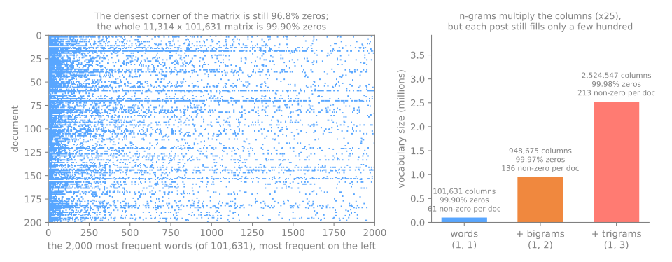
The right panel is the price of n-grams on the whole corpus: bigrams multiply the columns by 9, trigrams by 25, while each post fills only a few hundred of them. Most word pairs occur once in the whole corpus. min_df=2 (keep only terms present in at least 2 documents) or max_features keep the size under control.
What raw counts put first
Sum each column and sort: which words does a bag-of-words consider most important?
for params in [{}, {'stop_words': 'english'}]:
    cv = CountVectorizer(**params)
    Xc = cv.fit_transform(news.data)
    freq = np.asarray(Xc.sum(axis=0)).ravel()
    top = np.argsort(-freq)[:8]
    print(params, list(cv.get_feature_names_out()[top]))
    print(f"    '{cv.get_feature_names_out()[top[0]]}' occurs {freq[top[0]]:,} times, in {(Xc[:, top[0]] > 0).sum():,} posts")
{} ['the', 'ax', 'to', 'of', 'and', 'in', 'is', 'that']
    'the' occurs 106,381 times, in 9,475 posts
{'stop_words': 'english'} ['ax', 'max', 'people', 'like', 'don', 'just', 'know', 'use']
    'ax' occurs 62,387 times, in 20 posts
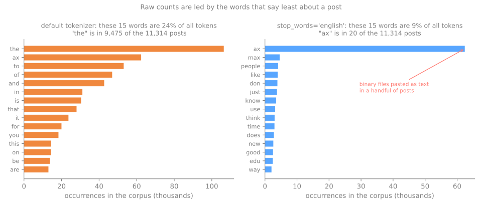
Two lessons in one figure. On the left, the columns with the largest counts are the, to, of, and: words present in almost every post ("the" in 9,475 of 11,314), which say nothing about the subject. An English stop list removes them. On the right, the new leader is "ax": 62,387 occurrences, in only 20 posts. Those posts contain binary files pasted as text, where "ax" repeats thousands of times. Raw counts let one strange document dominate the whole column. Both problems have the same cure, which is the subject of the next page: weigh each word by how many documents contain it, not only by how often it occurs.
Simulator: build the bag yourself
Type one document per line and watch the vocabulary and the count matrix update. The rules are scikit-learn's: lowercase, tokens of two or more letters or digits, stop words removed before the bigrams. The presets reproduce the examples of this page.
Things to try:
- word order: the first two sentences get identical vectors (the simulator flags "d1 = d2"). Tick add bigrams and they separate;
- sábado/sábados: three sentences about the same thing, and the singular, plural and capitalized forms of the same words land in different columns once you untick lowercase;
- binary: in the lesson preset, only d3 changes (gato 2 → 1).
Exercises
- By hand, compute the cosine between d2 and d3 of the table above, and check the value 0.365.
- Add the document "O peixe dorme." to the three of the lesson. How many columns does the vocabulary have now? Write the new row by hand, then check with
CountVectorizer. - A post of 300 words and a post of 30 words are about the same subject. Why can their Euclidean distance be large while their cosine is high? What changes if you use
binary=True? - With
ngram_range=(1, 3), how many columns do the three documents of the lesson produce? Count by hand first.
Lab: bag-of-words on real posts
Four newsgroups of the 20 Newsgroups collection (computer graphics, baseball, electronics and Christianity), about 2,100 posts. The lab builds the count matrix, looks at what it contains, and measures how each choice (stop words, min_df, binary, bigrams, character n-grams) changes the answer to one question: are the most similar posts about the same subject? It uses only scikit-learn and runs in well under a minute.
Run the blocks in order, in one session. To work on it directly, download the lab notebook and open it in Jupyter or Colab (File → Upload notebook).
Step 1 — load the posts
import numpy as np
import pandas as pd
from sklearn.datasets import fetch_20newsgroups

cats = ['comp.graphics', 'rec.sport.baseball', 'sci.electronics', 'soc.religion.christian']
raw = fetch_20newsgroups(subset='train', categories=cats,
                         remove=('headers', 'footers', 'quotes'), random_state=0)
keep = [i for i, t in enumerate(raw.data) if len(t.split()) >= 20]   # drop empty/very short posts
docs = [raw.data[i] for i in keep]
y = raw.target[keep]
names = np.array(raw.target_names)

print(f"{len(raw.data)} posts downloaded, {len(docs)} kept")
print(pd.Series(names[y]).value_counts().sort_index())
print(f"words per post: median {np.median([len(d.split()) for d in docs]):.0f}")
print(' '.join(docs[0].split())[:160])
2371 posts downloaded, 2116 kept
comp.graphics             521
rec.sport.baseball        495
sci.electronics           535
soc.religion.christian    565
Name: count, dtype: int64
words per post: median 97
Their phone number is 1-800-377-9777. The last catalog shows three Oaks jerseys: 36 Home, 42 Home, 39 Home - they're each $165.00. All their merchandise is hand
Of the 2,371 posts, 2,116 have at least 20 words once headers, signatures and quoted replies are removed; many of the others are empty. The four groups are balanced (495 to 565 posts) and a median post has 97 words. Removing the headers matters: they carry e-mail addresses and organizations, and anything that compares posts could match the senders instead of the subject. The first post, about baseball jerseys, shows what a document looks like: informal, with numbers and prices.
Step 2 — the count matrix
from sklearn.feature_extraction.text import CountVectorizer

counts = CountVectorizer()
C = counts.fit_transform(docs)
vocab = counts.get_feature_names_out()
freq = np.asarray(C.sum(axis=0)).ravel()

print(C.shape, f"{1 - C.nnz / (C.shape[0] * C.shape[1]):.2%} zeros")
print(f"distinct words per post (median): {np.median(np.diff(C.indptr)):.0f}")
print('10 most frequent words:', list(vocab[np.argsort(-freq)[:10]]))
print(f"words seen only once: {(freq == 1).mean():.0%} of the vocabulary")
(2116, 25715) 99.62% zeros
distinct words per post (median): 67
10 most frequent words: ['the', 'to', 'of', 'and', 'is', 'in', 'that', 'it', 'for', 'you']
words seen only once: 45% of the vocabulary
How to read it:
- 2,116 posts × 25,715 words, 99.62% zeros: a median post uses 67 distinct words out of 25,715.
- The ten most frequent words are all function words: "the", "to", "of" are in almost every post and say nothing about the subject.
- 45% of the vocabulary appears once in the whole corpus: the long tail of names, numbers, typos and rare words that Zipf's law predicts (overview).
Step 3 — what each newsgroup talks about
cv_stop = CountVectorizer(stop_words='english')
S = cv_stop.fit_transform(docs)
words = cv_stop.get_feature_names_out()
for c in range(4):
    total = np.asarray(S[y == c].sum(axis=0)).ravel()      # add up the rows of one group
    print(f"{names[c]:24s}", list(words[np.argsort(-total)[:8]]))
comp.graphics            ['image', 'graphics', 'edu', 'jpeg', 'file', 'use', 'data', 'files']
rec.sport.baseball       ['year', 'game', 'good', 'team', 'think', 'don', '00', 'just']
sci.electronics          ['use', 'like', 'power', 'don', 'wire', 'ground', 'used', 'know']
soc.religion.christian   ['god', 'jesus', 'people', 'church', 'think', 'does', 'know', 'believe']
Once the English stop words are removed, summing the rows of each group gives a readable portrait of it: image, graphics, jpeg, file for graphics; game, team, year for baseball; power, wire, ground for electronics; god, jesus, church, believe for Christianity. The bag-of-words does carry the subject. It also carries noise that a stop list does not catch: "don" (what the tokenizer leaves of "don't"), "think", "just", "use", "edu" (from e-mail addresses) and "00" (from baseball statistics) are frequent in some groups without being about anything.
Step 4 — shrinking the vocabulary
for params in [{}, {'stop_words': 'english'}, {'min_df': 2}, {'stop_words': 'english', 'min_df': 2},
               {'max_df': 0.5}]:
    cv = CountVectorizer(**params).fit(docs)
    print(f"{str(params):42s} {len(cv.vocabulary_):6d} columns")

cv_half = CountVectorizer(max_df=0.5).fit(docs)
print('dropped by max_df=0.5:', sorted(set(vocab) - set(cv_half.vocabulary_)))
{}                                          25715 columns
{'stop_words': 'english'}                   25411 columns
{'min_df': 2}                               12297 columns
{'stop_words': 'english', 'min_df': 2}      12001 columns
{'max_df': 0.5}                             25703 columns
dropped by max_df=0.5: ['and', 'be', 'for', 'have', 'in', 'is', 'it', 'of', 'that', 'the', 'this', 'to']
The knobs act on opposite ends of the frequency scale:
- the stop list removes only 304 columns (25,715 → 25,411), but they are the most frequent words;
min_df=2removes more than half of the vocabulary (→ 12,297): words present in a single post, which cannot help compare two posts;max_df=0.5drops the words present in more than half of the posts. Here that is only 12 words, all of them function words ("and", "the", "of", ...): a stop list learned from the data itself, without choosing a language.
Step 5 — comparing posts: counts, presence, stop words
from sklearn.neighbors import NearestNeighbors

def agreement(V, k=5):
    """Share of each post's k nearest posts (cosine) that come from the same newsgroup."""
    nn = NearestNeighbors(n_neighbors=k + 1, metric='cosine').fit(V)
    _, idx = nn.kneighbors(V)
    return (y[idx[:, 1:]] == y[:, None]).mean()

print(f"chance level: {np.sum(np.bincount(y) ** 2) / len(y) ** 2:.3f}")
for params in [{}, {'binary': True}, {'stop_words': 'english'}, {'stop_words': 'english', 'binary': True}]:
    V = CountVectorizer(**params).fit_transform(docs)
    print(f"{str(params):42s} agreement {agreement(V):.3f}")
chance level: 0.251
{}                                         agreement 0.490
{'binary': True}                           agreement 0.650
{'stop_words': 'english'}                  agreement 0.793
{'stop_words': 'english', 'binary': True}  agreement 0.768
A way to score a representation without training any model: for every post, find its 5 nearest posts by cosine and count how many come from the same newsgroup. Picking neighbors at random would give 0.251 (the chance that two random posts share a group).
- Raw counts: 0.490. Posts are "near" when they use the, to, of in similar proportions, which has little to do with the subject.
binary=True: 0.650. Presence limits how much a repeated function word can weigh, and the score jumps.- Stop words removed: 0.793. Removing the function words helps most. With them gone, counts (0.793) are slightly better than presence (0.768): once the words that remain are about something, repeating them is informative.
The TF-IDF page goes further, weighing every word by how many posts contain it instead of removing a fixed list.
Step 6 — n-grams of words and of characters
for params in [{'stop_words': 'english', 'min_df': 2},
               {'stop_words': 'english', 'min_df': 2, 'ngram_range': (1, 2)},
               {'analyzer': 'char_wb', 'ngram_range': (3, 5), 'min_df': 2}]:
    V = CountVectorizer(**params).fit_transform(docs)
    print(f"{str(params):70s} {V.shape[1]:6d} columns · agreement {agreement(V):.3f}")
{'stop_words': 'english', 'min_df': 2}                                  12001 columns · agreement 0.793
{'stop_words': 'english', 'min_df': 2, 'ngram_range': (1, 2)}           25184 columns · agreement 0.793
{'analyzer': 'char_wb', 'ngram_range': (3, 5), 'min_df': 2}             94920 columns · agreement 0.529
Bigrams double the vocabulary (12,001 → 25,184 columns) and do not change the agreement (0.793 both ways): telling baseball from electronics is a matter of vocabulary, which single words already capture. Character n-grams of 3 to 5 letters give 94,920 columns and a worse agreement (0.529): their pieces are shared by words of every subject, and they include the pieces of the function words that the stop list had removed. They pay off elsewhere: short and noisy texts, typos, languages with rich morphology.
Step 7 — the bag cannot tell a post from its shuffled words
rng = np.random.default_rng(0)
analyzer = counts.build_analyzer()
shuffled = [' '.join(rng.permutation(analyzer(d))) for d in docs[:3]]
print(shuffled[0][:120])

A = counts.transform(docs[:3])
B = counts.transform(shuffled)
print('same count vectors:', (A != B).nnz == 0)
42 couple merchandise last wool 165 on 800 if call shows number also replica home jackets three even and they 39 afford
same count vectors: True
The first post with its words shuffled is unreadable, and its count vector is exactly the same as the original's, as are those of the next two posts: (A != B).nnz == 0 checks that no cell differs. Everything a bag-of-words knows about a document survives a random shuffle of its words.
Your turn
- Most similar posts. Pick a post, compute
cosine_similarity(V[i], V)with the best representation of step 5, and print the three most similar posts with their newsgroup. Do the same with raw counts. Which words make the raw-count neighbors "similar"? - Your own stop list. Add the words of step 4's
max_df=0.5list and the most frequent non-topical words of step 3 ("don", "just", "think") to scikit-learn's English list, and rerun step 5. Does the agreement go up? - Portuguese. Write five short sentences in Portuguese about two different subjects, and build their bag with and without the tiny stop list of the overview. Which words does the default tokenizer drop before any stop list is applied?
- Shuffled with bigrams. Repeat step 7 with
CountVectorizer(ngram_range=(1, 2)). Are the vectors still the same? Why?
Class materials
Lab notebook
The lab of this page as a notebook, ready for Jupyter or Colab: lab notebook.
References
- Harris, Z. S. "Distributional Structure." Word 10, no. 2–3 (1954): 146–162 — where "language is not merely a bag of words" appears. DOI
- Salton, G.; Wong, A.; Yang, C. S. "A Vector Space Model for Automatic Indexing." Communications of the ACM 18, no. 11 (1975): 613–620 — documents as vectors, one axis per term. DOI
- Lang, K. "NewsWeeder: Learning to Filter Netnews." Proceedings of ICML (1995): 331–339 — the origin of the 20 Newsgroups collection. DOI
- Manning, C. D.; Raghavan, P.; Schütze, H. Introduction to Information Retrieval. Cambridge University Press (2008) — chapter 2 (tokens and terms) and chapter 6 (the vector space model). Full text