U4.4 Sentence Embeddings
Word embeddings give every word a dense vector, but most tasks are about texts: find the FAQ entry that answers a question, group support tickets, retrieve the documents that match a query. This page is about one vector per sentence or short document, arranged so that the cosine between two of them tracks how close their meanings are.
The simplest answer, averaging the word vectors, is built by hand first, and its failures are measured: word order and negation vanish, and every sentence ends up looking like every other. Then contextual embeddings: a Transformer computes the vector of each word from the whole sentence around it, so "bank" next to "river" and "bank" next to "loan" get different vectors. Sentence-BERT trains such a network so that one vector summarizes a sentence, and the sentence-transformers library makes it a one-line call. With it: TF-IDF, averaged word vectors and sentence embeddings compared on the same pairs, English and Portuguese models compared on Portuguese, semantic search as nearest neighbors, sentences grouped with k-means, and the practical details (length limits, cost, choosing a model). The overview puts TF-IDF and sentence embeddings side by side on search and classification; this page opens the box. Every number below comes from running the code next to it.
The page follows one pipeline in four stages, drawn below: 1. average the words, the simplest sentence vector, and what it loses; 2. words in context, where a Transformer gives each word a vector that depends on the sentence; 3. one vector per sentence, with Sentence-BERT, compared against TF-IDF and averaging; 4. search and group, using those vectors for semantic search, clustering and in practice. Each stage links to its section, and in the slides a strip at the bottom shows which stage you are in.
- Average the wordsmean of GloVe vectors; order and negation vanish
- Words in contextTransformers: one word, several vectors
- One vector per sentenceSentence-BERT against TF-IDF and averaging; other languages
- Search and groupsemantic search, clustering, practical notes
Slides
Click the slides and use the ← → arrows to navigate; F goes full screen and Esc shows every slide. Open the slides in a new tab
From word vectors to a sentence vector
Averaging, by hand
Stage 1. A sentence is a sequence of words and each word has a vector, so the obvious sentence vector is the mean of its word vectors. With the GloVe vectors of the previous page:
import re
import numpy as np
import pandas as pd
import gensim.downloader as api

glove = api.load('glove-wiki-gigaword-50')          # the word vectors of the previous page

def words_of(text):
    return [w for w in re.findall(r"[a-z]+", text.lower()) if w in glove.key_to_index]

def avg_vector(text):
    return np.mean([glove[w] for w in words_of(text)], axis=0)

s = "the movie was great"
for w in words_of(s):
    print(f"{w:6s}", glove[w][:4].round(3), '...')
print('mean  ', avg_vector(s)[:4].round(3), '...  <- one vector for the sentence')
the    [ 0.418  0.25  -0.412  0.122] ...
movie  [ 0.308  0.172 -0.233  0.023] ...
was    [ 0.087 -0.194 -0.243 -0.334] ...
great  [-0.027  1.336 -1.028 -0.373] ...
mean   [ 0.197  0.391 -0.479 -0.141] ...  <- one vector for the sentence
Check the first column with a calculator: \((0.418 + 0.308 + 0.087 - 0.027) / 4 = 0.1965\), printed as 0.197. Each of the 50 coordinates is averaged the same way, and the sentence gets a vector of the same size as a word. It costs nothing, needs no training, and works for any sentence whose words are in the vocabulary.
What averaging loses
def cos(u, v):
    return float(u @ v / (np.linalg.norm(u) * np.linalg.norm(v)))

for a, b in [("the dog bit the man", "the man bit the dog"),
             ("the movie was good", "the movie was not good"),
             ("the movie was great", "the film was excellent"),
             ("the stock market fell sharply today", "my cat likes to sleep on the couch")]:
    print(f"{cos(avg_vector(a), avg_vector(b)):.2f}   {a}  /  {b}")
1.00   the dog bit the man  /  the man bit the dog
0.99   the movie was good  /  the movie was not good
0.96   the movie was great  /  the film was excellent
0.66   the stock market fell sharply today  /  my cat likes to sleep on the couch
Three failures, all structural:
- Order is gone. "The dog bit the man" and "the man bit the dog" contain the same words, so their means are identical: cosine 1.00, exactly. An average, like a bag of words, is blind to order.
- Negation barely registers. "not" is one word out of five, and its vector is averaged with the others: 0.99.
- Everything looks similar. Two sentences with nothing in common, about the stock market and a sleepy cat, still score 0.66, while a true paraphrase scores 0.96. The frequent words ("the", "was", "my", "on") pull every average toward the same "average English" direction, and the whole scale is squeezed into its top third.
Weighting the words by their idf (see TF-IDF) before averaging helps with the last problem, and the average is a surprisingly strong baseline for grouping texts by topic. But nothing done after the words are looked up can fix the first two: each word's vector was fixed before it met the sentence.
Contextual embeddings
Transformers, in one paragraph
Stage 2. A Transformer (Vaswani et al., 2017) is a neural network that reads a whole sentence at once. It first cuts the text into subword tokens from a fixed vocabulary of about 30,000 pieces, so no word is ever out of vocabulary, and gives each token a starting vector. Then, in each of its layers, every token's vector is recomputed as a weighted mix of the vectors of all the tokens in the sentence, with weights the network computes from the tokens themselves (the mechanism is called attention). After a few layers, the vector of "bank" has absorbed information from "river" or from "loan", depending on which is there. BERT (Devlin et al., 2019) is a Transformer trained on billions of words to fill in hidden words from their context, and it produces one contextual vector per token. How these networks are built and trained is the subject of Neural Networks and of the Deep Learning course; here they are used as a black box that turns text into vectors.
One word, several vectors
sentence-transformers loads such a network. The small English model all-MiniLM-L6-v2 (6 layers) shows the tokenizer and, with output_value='token_embeddings', the vector of every token. Take the vector of the token "bank" in six sentences, three about rivers and three about money:
from sentence_transformers import SentenceTransformer

model = SentenceTransformer('all-MiniLM-L6-v2')      # ~90 MB, downloaded once
print(model.tokenizer.tokenize("Embeddings are unbelievably useful"))

bank = ["we had a picnic on the bank of the river", "the boat drifted toward the muddy bank",
        "fish hide under the grassy bank", "she went to the bank to get a loan",
        "the bank raised its interest rates", "he deposited the check at the bank"]
vecs = []
for s in bank:
    tokens = model.tokenizer.convert_ids_to_tokens(model.tokenizer(s)['input_ids'])
    token_vecs = model.encode(s, output_value='token_embeddings')     # one vector per token
    vecs.append(np.asarray(token_vecs[tokens.index('bank')].cpu()))
V = np.array(vecs) / np.linalg.norm(vecs, axis=1, keepdims=True)
labels = ['river 1', 'river 2', 'river 3', 'money 4', 'money 5', 'money 6']
print(pd.DataFrame(V @ V.T, index=labels, columns=labels).round(2))
['em', '##bed', '##ding', '##s', 'are', 'un', '##bel', '##ie', '##va', '##bly', 'useful']
         river 1  river 2  river 3  money 4  money 5  money 6
river 1     1.00     0.83     0.86     0.76     0.76     0.76
river 2     0.83     1.00     0.84     0.72     0.72     0.73
river 3     0.86     0.84     1.00     0.72     0.73     0.71
money 4     0.76     0.72     0.72     1.00     0.88     0.86
money 5     0.76     0.72     0.73     0.88     1.00     0.82
money 6     0.76     0.73     0.71     0.86     0.82     1.00
The first line is the tokenizer at work: "embeddings" becomes em + ##bed + ##ding + ##s and "unbelievably" five pieces (## marks a piece that continues a word). The matrix is the point. In GloVe, "bank" has one vector and all 36 cells would be 1.00. Here every river "bank" is closer to the other river "banks" (0.83 to 0.86) than to any money "bank" (0.71 to 0.76), and the money "banks" are closest to each other (0.82 to 0.88). The same token gets a different vector in each sentence, and the difference follows the sense. This is what "contextual" means, and it is exactly the limit of the previous page.
Sentence-BERT
Trained to compare sentences
Stage 3. A contextual model gives one vector per token. To get one per sentence, the usual step is mean pooling: average the token vectors, as we averaged GloVe vectors, except that now each token vector already carries its context. BERT itself was not trained for this, and the cosine between averaged BERT vectors tracks meaning poorly. Sentence-BERT (Reimers & Gurevych, 2019) adds a second training stage: pass two sentences through the same network, pool each into a vector, and adjust the network so that the cosine is high for pairs that mean the same thing and low for pairs that do not, over hundreds of thousands (in later models, over a billion) of labeled or naturally paired examples.
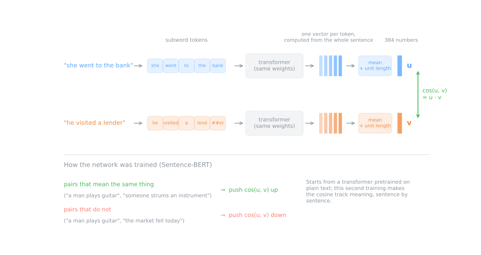
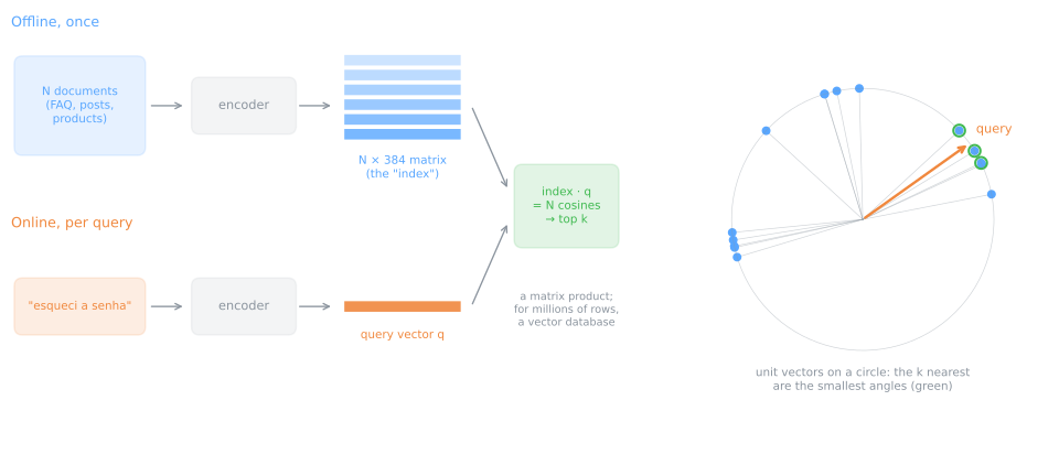
Because each sentence is encoded separately (a bi-encoder), a collection can be encoded once and stored; comparing a new sentence with a million stored ones is then one matrix product, which is what makes semantic search practical.
Using sentence-transformers
all-MiniLM-L6-v2, loaded above, is a Sentence-BERT model: encode returns one vector per text, already pooled.
E = model.encode(["the movie was great", "the film was excellent", "the stock market fell sharply today"],
                 normalize_embeddings=True)
print(E.shape, '· length of each row:', np.linalg.norm(E, axis=1).round(3))
print(E[0, :6].round(3), '...')
print((E @ E.T).round(2))
print(f"{sum(p.numel() for p in model.parameters()):,} parameters · reads at most {model.max_seq_length} tokens")
(3, 384) · length of each row: [1. 1. 1.]
[-0.135  0.066 -0.065 -0.011 -0.017  0.013] ...
[[1.   0.88 0.04]
 [0.88 1.   0.04]
 [0.04 0.04 1.  ]]
22,713,216 parameters · reads at most 256 tokens
How to read it:
- Each text is 384 numbers. None of them means anything on its own; only distances do.
normalize_embeddings=Truemakes every row length 1, so the dot productE @ E.Tis the cosine matrix. Always normalize when you will compare vectors; it also makes Euclidean distance and cosine rank neighbors identically.- The two paraphrases score 0.88, with only "the" and "was" in common; the stock market sentence scores 0.04 with both. Compare with the averaged GloVe vectors above (0.96 against 0.66): the scale is now used from bottom to top.
- 22.7 million parameters, 256 tokens. The model is small by current standards (about 90 MB) and reads at most 256 tokens; anything after that is cut, as the practical notes measure.
Three representations, the same pairs
TF-IDF, averaged GloVe vectors and Sentence-BERT on eight pairs chosen to probe one property each. The TF-IDF is fitted on the 16 sentences of the table:
from sklearn.feature_extraction.text import TfidfVectorizer

pairs = {'paraphrase':               ("the movie was great", "the film was excellent"),
         'paraphrase, other words':  ("a man is playing a guitar", "someone is strumming an instrument"),
         'same need, other words':   ("how do I reset my password", "I forgot my login credentials"),
         'negation':                 ("the movie was good", "the movie was not good"),
         'word order':               ("the dog bit the man", "the man bit the dog"),
         'bank: river vs money':     ("she sat on the river bank", "she went to the bank to get a loan"),
         'apple: company vs fruit':  ("apple released a new phone", "i ate an apple and a banana"),
         'unrelated':                ("the stock market fell sharply today", "my cat likes to sleep on the couch")}
tfidf = TfidfVectorizer().fit([s for pair in pairs.values() for s in pair])
rows = {}
for name, (a, b) in pairs.items():
    t = tfidf.transform([a, b]).toarray()
    e = model.encode([a, b], normalize_embeddings=True)
    rows[name] = {'TF-IDF': cos(t[0], t[1]), 'avg GloVe': cos(avg_vector(a), avg_vector(b)),
                  'SBERT': float(e[0] @ e[1])}
print(pd.DataFrame(rows).T.round(2))
                         TF-IDF  avg GloVe  SBERT
paraphrase                 0.28       0.96   0.88
paraphrase, other words    0.19       0.92   0.56
same need, other words     0.15       0.92   0.68
negation                   0.82       0.99   0.82
word order                 1.00       1.00   0.98
bank: river vs money       0.29       0.92   0.60
apple: company vs fruit    0.18       0.87   0.23
unrelated                  0.04       0.66   0.02
Read the columns one at a time, then the rows.
- TF-IDF measures shared words. The paraphrases without shared content words score 0.15 to 0.28, not far above the unrelated pair (0.04), while the negation (0.82) and the word-order swap (1.00) look almost identical.
- Averaged GloVe says "similar" to everything: 0.66 for the unrelated pair, 0.87 to 1.00 for the rest. It does rank the unrelated pair last, but its range is so narrow that no threshold separates related from unrelated with confidence.
- Sentence-BERT uses the whole scale: 0.02 for unrelated, 0.88 for the paraphrase, 0.56 and 0.68 for paraphrases with no word in common. And the polysemy rows come apart: "apple" the company and "apple" the fruit score 0.23, because each "apple" was read in its sentence.
- What none of them fixes. Negation stays high (0.82): "the movie was good" and "the movie was not good" are about the same film and the same quality, and a model trained on "are these two sentences about the same thing?" says yes. Word order barely moves (0.98): mean pooling blurs who did what to whom, even when each token vector saw its context. If your task depends on negation or roles (sentiment, contradictions, who is liable), check it explicitly.
The overview runs the same kind of comparison on Portuguese sentences with the multilingual model, with the same conclusions.
Other languages
all-MiniLM-L6-v2 was trained on English. A multilingual model, paraphrase-multilingual-MiniLM-L12-v2, was trained with the method of Reimers & Gurevych (2020): a student network learns to put a sentence and its translations at the point where an English teacher model puts the English sentence, for 50+ languages. The difference, on Portuguese:
multi = SentenceTransformer('paraphrase-multilingual-MiniLM-L12-v2')   # 50+ languages, ~470 MB
pt_pairs = [("o filme foi ótimo", "o longa foi excelente"),              # paraphrase
            ("esqueci minha senha", "não lembro a senha da conta"),       # paraphrase
            ("o filme foi ótimo", "the movie was great"),                 # translation
            ("o filme foi ótimo", "a bolsa de valores caiu hoje")]        # unrelated
for a, b in pt_pairs:
    e_en = model.encode([a, b], normalize_embeddings=True)
    e_mu = multi.encode([a, b], normalize_embeddings=True)
    print(f"English-only {e_en[0] @ e_en[1]:.2f} · multilingual {e_mu[0] @ e_mu[1]:.2f}   {a} / {b}")
English-only 0.65 · multilingual 0.66   o filme foi ótimo / o longa foi excelente
English-only 0.40 · multilingual 0.81   esqueci minha senha / não lembro a senha da conta
English-only 0.08 · multilingual 0.98   o filme foi ótimo / the movie was great
English-only 0.40 · multilingual -0.02   o filme foi ótimo / a bolsa de valores caiu hoje
The English model does not fail loudly: it returns numbers for Portuguese too, because its subword pieces can spell anything. But look at its scores: "I forgot my password" / "I don't remember the account password" scores 0.40, and "the film was great" / "the stock market fell today", which have nothing in common, also score 0.40. A model that gives the same score to a paraphrase and to an unrelated pair is useless for search in that language. The multilingual model separates them (0.81 against −0.02), and it puts a Portuguese sentence and its English translation at 0.98, so a Portuguese query can find English documents. Choose a model trained on your language; the lab measures this on 2,448 pairs rated by people.
Semantic search is k-nearest neighbors
Stage 4. The most common use of sentence embeddings is semantic search: encode a collection once, encode each query, return the documents whose vectors are nearest. It is the same nearest-neighbor search that underlies the k-NN classifier, a lesson that comes later in the course; here it is used only to find neighbors, with no labels and no prediction. scikit-learn's NearestNeighbors with metric='cosine' does it (it reports the cosine distance, \(1 - \cos\)):
from sklearn.neighbors import NearestNeighbors

faq = ["Como faço para trocar a senha da minha conta?",
       "Qual é o prazo de entrega para o Nordeste?",
       "Posso devolver um produto depois de usado?",
       "Quais são as formas de pagamento aceitas?",
       "Como rastrear o meu pedido?",
       "O produto tem garantia contra defeitos de fábrica?",
       "Como emitir a segunda via da nota fiscal?",
       "Como cancelar uma compra que ainda não foi enviada?"]
E_faq = multi.encode(faq, normalize_embeddings=True)            # encode the collection once
index = NearestNeighbors(n_neighbors=2, metric='cosine').fit(E_faq)

queries = ["esqueci minha senha", "onde está minha encomenda?", "dá pra pagar com pix?",
           "desisti da compra", "o celular veio com defeito", "I need a copy of my invoice"]
dist, ids = index.kneighbors(multi.encode(queries, normalize_embeddings=True))
for q, d, i in zip(queries, dist, ids):
    print(f"{q}\n   1st {1 - d[0]:.2f} {faq[i[0]]}\n   2nd {1 - d[1]:.2f} {faq[i[1]]}")
esqueci minha senha
   1st 0.68 Como faço para trocar a senha da minha conta?
   2nd 0.33 Como rastrear o meu pedido?
onde está minha encomenda?
   1st 0.60 Como rastrear o meu pedido?
   2nd 0.40 Qual é o prazo de entrega para o Nordeste?
dá pra pagar com pix?
   1st 0.42 Quais são as formas de pagamento aceitas?
   2nd 0.32 Como faço para trocar a senha da minha conta?
desisti da compra
   1st 0.62 Como cancelar uma compra que ainda não foi enviada?
   2nd 0.43 Posso devolver um produto depois de usado?
o celular veio com defeito
   1st 0.26 Posso devolver um produto depois de usado?
   2nd 0.24 O produto tem garantia contra defeitos de fábrica?
I need a copy of my invoice
   1st 0.43 Como faço para trocar a senha da minha conta?
   2nd 0.40 Como rastrear o meu pedido?
Four of the six queries get the right answer first, although "encomenda" (parcel) is not "pedido" (order) and "desisti" (I gave up) is not "cancelar" (cancel). The two misses are worth reading:
- "o celular veio com defeito" (the phone arrived broken): the model's first choice is the return policy, and the warranty question is second. Both are defensible answers, and the scores are low and close (0.26 and 0.24): the model is unsure, and a system should say so instead of answering.
- "I need a copy of my invoice": the right entry is "segunda via da nota fiscal", literally "second copy of the tax receipt", a Brazilian expression the model does not connect to "copy of my invoice". Idioms and domain jargon are where general-purpose embeddings fail.
The simulator below makes the comparison with TF-IDF tangible. It holds 40 sentences in Portuguese and English (account, delivery, payment, refunds, three kinds of banco, weather, cooking, football) and 10 queries, with a ✓ on the answers a person would accept. The sentence embeddings were computed in advance with the multilingual model; the TF-IDF ranking is computed in your browser. You can also type your own query, which only TF-IDF can process without the network.
Over the ten queries, the embeddings put 15 of the 19 relevant sentences in their top 3, TF-IDF 6. The query "erro 402" is the exception worth remembering: the rare token "402" gives TF-IDF a clean win, while the embedding ranks "erro 404" first. The overview measures this effect on error codes; production search engines combine both rankings (hybrid search). The simulator's data was produced by a short script next to this page, which also prints the reference TF-IDF ranking computed with scikit-learn; the embeddings are stored as 8-bit integers, which changes no cosine by more than 0.002.
Clustering sentences
Sentence vectors are ordinary numeric rows, so everything from clustering applies. Sixteen Portuguese headlines from four subjects (football, cooking, economy, weather), grouped with k-means into four clusters, once on TF-IDF and once on embeddings, scored with the adjusted Rand index (ARI) against the true subjects:
from sklearn.cluster import KMeans
from sklearn.metrics import adjusted_rand_score

texts = ["O Flamengo venceu o clássico no Maracanã", "O atacante marcou dois gols no segundo tempo",
         "A seleção perdeu nos pênaltis", "O técnico foi demitido após a derrota",
         "Misture a farinha com os ovos e o leite", "Asse o bolo por quarenta minutos",
         "Tempere o frango com alho e limão", "A receita leva manteiga e açúcar",
         "O banco central subiu a taxa de juros", "A inflação de março ficou acima do esperado",
         "O dólar fechou em queda nesta sexta", "Os investidores venderam ações da Petrobras",
         "Vai chover forte no fim de semana", "A frente fria derrubou as temperaturas",
         "O verão deve ser mais quente que o normal", "Alerta de tempestade para o litoral"]
topic = np.repeat([0, 1, 2, 3], 4)                  # football, cooking, economy, weather
X_tfidf = TfidfVectorizer().fit_transform(texts)
X_emb = multi.encode(texts, normalize_embeddings=True)
for name, X in [('TF-IDF', X_tfidf), ('embeddings', X_emb)]:
    labels = KMeans(n_clusters=4, n_init=10, random_state=0).fit_predict(X)
    print(f"{name:10s} ARI {adjusted_rand_score(topic, labels):.2f}   clusters: {labels}")
TF-IDF     ARI 0.02   clusters: [1 1 3 0 2 0 2 0 0 0 0 2 1 0 0 0]
embeddings ARI 0.68   clusters: [2 2 2 2 0 0 0 0 3 3 1 2 1 1 1 1]
On TF-IDF the ARI is 0.02, no better than chance. The headlines are short and the four in each subject share almost no words, so every TF-IDF vector is nearly orthogonal to every other, and k-means has nothing to work with: it puts nine of the sixteen in one cluster. On the embeddings the ARI is 0.68. Football, cooking and weather come out whole; the economy headlines are split, with "investors sold Petrobras shares" joining football and "the dollar closed lower" joining weather. Short texts are where sentence embeddings help clustering most, and Topic Modeling & BERTopic builds a whole method on this: embed, reduce with UMAP, cluster with HDBSCAN.
Practical notes
Normalize. Pass normalize_embeddings=True (or divide each row by its norm) whenever you compare vectors. Then cosine is a dot product, a whole similarity matrix is one E @ E.T, and every nearest-neighbor tool gives the same ranking with Euclidean or cosine distance.
Encode in batches, once. model.encode(list_of_texts, batch_size=64) processes the texts in groups, which is much faster than one call per text. Encode a collection once, save the matrix (np.save), and encode only new texts afterwards.
Mind the length limit. A model reads at most max_seq_length tokens and silently drops the rest:
long_text = " ".join(["The committee discussed the budget for the next fiscal year."] * 30)
changed = long_text + " In the end, the committee decided to close the whole department."
print(len(model.tokenizer.tokenize(long_text)), 'tokens in the long text')
e = model.encode([long_text, changed], normalize_embeddings=True)
print(f"cosine between the text and the text + a decisive last sentence: {e[0] @ e[1]:.4f}")
The text already has 330 tokens, more than the 256 this model reads, so the decisive last sentence changes nothing: cosine 1.0000. For long documents, split them into paragraphs or chunks, embed each, and search over chunks (or average the chunk vectors for a document-level vector). The multilingual model is stricter still: 128 tokens.
Know the cost. all-MiniLM-L6-v2 has 22.7 million parameters; the multilingual model has 117.7 million (lab). Encoding runs a network forward pass for each text, so it takes seconds to minutes on a CPU for thousands of texts, where TF-IDF takes a fraction of a second, and a GPU speeds it up by an order of magnitude. Storage is 384 × 4 bytes = 1.5 KB per text in float32.
Choose the model for the job. Three questions: which language? (an English-only model scored a paraphrase and an unrelated pair the same in Portuguese); which kind of text? (models trained on web questions and answers are good at search; legal or medical jargon may need a domain model); how much can you pay? (bigger models are better and slower). The MTEB benchmark (Muennighoff et al., 2023) ranks hundreds of embedding models on dozens of tasks and languages; use it to shortlist, then measure on a sample of your own data, as the lab does.
Scale with an index. For a few thousand texts, a matrix product is instant. For millions, vector databases keep the embeddings in approximate nearest-neighbor indexes that answer in milliseconds; they are the retrieval half of the LLM systems in The Frontier.
Exercises
- Average the GloVe vectors of "the man bit the dog" and "the dog bit the man" by hand for one coordinate (use
glove['dog'][0]and friends). Why must every coordinate be identical, whatever the vectors are? - In the three-representation table, TF-IDF scores the negation pair 0.82 and SBERT also 0.82. Propose two sentences where you expect SBERT to score much lower than TF-IDF, and two where you expect the opposite. Run them.
- The FAQ search missed "I need a copy of my invoice". Add one FAQ entry, or rewrite one, so that this query finds it, without breaking the other five. What does this suggest about writing a knowledge base for semantic search?
- Change the clustering example to
n_clusters=5. Which headline moves, and does the ARI go up or down? Why is ARI usable here but not in a real clustering problem?
Lab: sentence similarity in Portuguese
Do sentence embeddings agree with people? ASSIN 2 (Real, Fonseca & Gonçalo Oliveira, 2020) is a Brazilian Portuguese benchmark: pairs of sentences, each rated by human annotators for how related they are, from 1 (unrelated) to 5 (same meaning). Its test set has 2,448 pairs. You will score every pair with TF-IDF and with two sentence-transformer models, measure how well each score follows the human one, look at where they disagree, and then use the embeddings of the 3,659 distinct sentences for search, clustering and a map.
The lab runs in about a minute on a laptop CPU after the model downloads (about 90 MB and 470 MB), most of it encoding the sentences twice; a Colab GPU runtime makes it a few seconds. Run the blocks in order, in one session. To work on it directly, download the lab notebook and open it in Jupyter or Colab (File → Upload notebook); in Colab, run !pip install sentence-transformers first.
Step 1 — load the pairs
# In Colab, run once:  !pip install sentence-transformers
import numpy as np
import pandas as pd

url = 'https://huggingface.co/api/datasets/nilc-nlp/assin2/parquet/default/test/0.parquet'
pairs = pd.read_parquet(url)[['premise', 'hypothesis', 'relatedness_score']]
pairs.columns = ['A', 'B', 'human']
sentences = list(dict.fromkeys(list(pairs.A) + list(pairs.B)))      # unique, in order
pos = {s: i for i, s in enumerate(sentences)}

print(len(pairs), 'pairs ·', len(sentences), 'distinct sentences')
print(pairs.human.describe().round(2).to_string())
with pd.option_context('display.max_colwidth', 60, 'display.width', 200):
    print(pairs.iloc[[1, 8, 53, 1906]].to_string())
2448 pairs · 3659 distinct sentences
count    2448.00
mean        3.57
std         1.00
min         1.00
25%         3.00
50%         3.75
75%         4.25
max         5.00
                                                        A                                             B  human
1                  O cara está fazendo exercícios no chão               Um cara está fazendo exercícios   3.75
8                        Uma mulher está andando a cavalo       Não tem nenhuma mulher andando a cavalo   3.30
53                       Uma mulher está andando a cavalo  Alguma coisa está sendo frita por uma mulher   1.10
1906  Algumas cebolas estão sendo cortadas por uma pessoa                      Um hamster está cantando   1.00
How to read it. 2,448 pairs built from 3,659 distinct sentences, so most sentences appear in more than one pair. The human score averages 3.57 and half the pairs are at 3.75 or above: the dataset leans toward related pairs. The four examples cover the range: a near-paraphrase (3.75), a negation rated 3.3 (a pair can be related without meaning the same thing: ASSIN 2 asks about relatedness), and two unrelated pairs at 1.1 and 1.0. The sentences are short descriptions of everyday scenes (people cooking, dogs running, men playing guitar), adapted from SICK-BR, a Portuguese version of the English SICK dataset.
Step 2 — TF-IDF as the baseline
from sklearn.feature_extraction.text import TfidfVectorizer

tfidf = TfidfVectorizer().fit(sentences)
T = tfidf.transform(sentences)                      # rows already have length 1
ia, ib = pairs.A.map(pos).to_numpy(), pairs.B.map(pos).to_numpy()
pairs['TF-IDF'] = np.asarray(T[ia].multiply(T[ib]).sum(axis=1)).ravel()   # row-wise dot = cosine
print(f"Spearman(TF-IDF cosine, human score) = {pairs['TF-IDF'].corr(pairs.human, method='spearman'):.3f}")
How to read it. Each sentence is encoded once and each pair looked up by position; the element-wise product summed along each row is the cosine, since TF-IDF rows have length 1. The score is compared with the human one using the Spearman correlation from EDA: it asks whether the pairs rank in the same order, which is what matters for search, and it does not care that a cosine and a 1–5 scale are in different units. 0.547 is a real but modest agreement: shared words are a decent proxy for relatedness in this dataset, because related pairs are often rewrites of the same caption.
Step 3 — two models scored against human judgments
from sentence_transformers import SentenceTransformer

models, emb = {}, {}
for name in ['all-MiniLM-L6-v2', 'paraphrase-multilingual-MiniLM-L12-v2']:
    models[name] = SentenceTransformer(name)
    emb[name] = models[name].encode(sentences, batch_size=64, normalize_embeddings=True)
    pairs[name] = np.sum(emb[name][ia] * emb[name][ib], axis=1)        # unit rows: dot = cosine
    print(f"{name:38s} {emb[name].shape}  Spearman {pairs[name].corr(pairs.human, method='spearman'):.3f}")
all-MiniLM-L6-v2                       (3659, 384)  Spearman 0.564
paraphrase-multilingual-MiniLM-L12-v2  (3659, 384)  Spearman 0.715
How to read it. The English-only model reaches 0.564, barely above TF-IDF (0.547): on Portuguese, it mostly sees shared subword pieces, which is what TF-IDF sees. The multilingual model reaches 0.715: same architecture family, same 384 numbers, but trained on Portuguese among 50+ languages. This is the "choose a model for your language" advice, measured on 2,448 human judgments. And neither model was trained on ASSIN 2: this is the score you get off the shelf.
Step 4 — where TF-IDF and embeddings disagree
E = emb['paraphrase-multilingual-MiniLM-L12-v2']
pairs['emb'] = pairs['paraphrase-multilingual-MiniLM-L12-v2']
cols = ['A', 'B', 'human', 'TF-IDF', 'emb']
with pd.option_context('display.max_colwidth', 60, 'display.width', 250):
    print('TF-IDF low, humans high (paraphrases with other words):')
    print(pairs[(pairs.human >= 4.5)].nsmallest(3, 'TF-IDF')[cols].round(2).to_string())
    print('\nnegations:')
    print(pairs[pairs.B.str.startswith('Não tem nenhum')].head(4)[cols].round(2).to_string())
TF-IDF low, humans high (paraphrases with other words):
                                            A                                                    B  human  TF-IDF   emb
1577  Uma senhora está fritando alguma comida  Alguns alimentos estão sendo fritos por uma senhora   4.50    0.11  0.84
2163           Está chovendo em um homem a pé                       Um homem está andando na chuva   4.90    0.13  0.90
1376     Um cara está conversando ao telefone                     Um cara está dando um telefonema   4.75    0.14  0.94

negations:
                                                       A                                                            B  human  TF-IDF   emb
8                       Uma mulher está andando a cavalo                      Não tem nenhuma mulher andando a cavalo    3.3    0.67  0.56
22  Um cachorro está correndo para cima do morro gramado  Não tem nenhum cachorro correndo para cima do morro gramado    3.0    0.88  0.60
38          Um homem está fatiando uma batata em pedaços          Não tem nenhum homem fatiando uma batata em pedaços    3.5    0.82  0.62
49                       Um homem está fatiando um peixe                       Não tem nenhum homem cortando um peixe    2.8    0.51  0.52
How to read it. The first table is where embeddings earn their cost: "a lady is frying some food" and "some food is being fried by a lady" (4.50 from people) share almost no word form (fritando/fritos, comida/alimentos), so TF-IDF gives 0.11, while the embedding gives 0.84. The same for "it is raining on a man on foot" / "a man is walking in the rain" (0.13 against 0.90). The second table shows the negations of ASSIN 2 ("Não tem nenhum..." = "there is no..."). People rate them 2.8 to 3.5, related but not equivalent; TF-IDF scores them high (up to 0.88) because almost every word is shared, and the embedding sits lower (0.52 to 0.62) but still well above unrelated pairs. Neither representation understands negation; the embedding is just less fooled by the shared words.
Step 5 — semantic search over 3,659 sentences
from sklearn.neighbors import NearestNeighbors

model = models['paraphrase-multilingual-MiniLM-L12-v2']
index = NearestNeighbors(n_neighbors=3, metric='cosine').fit(E)
queries = ['alguém está preparando comida', 'um animal correndo na areia', 'a person is playing music']
dist, ids = index.kneighbors(model.encode(queries, normalize_embeddings=True))
tf_scores = (tfidf.transform(queries) @ T.T).toarray()
for q, d, i, t in zip(queries, dist, ids, tf_scores):
    print(f"\n{q}")
    for dj, j in zip(d, i):
        print(f"   emb    {1 - dj:.2f}  {sentences[j]}")
    j = int(np.argmax(t))
    print(f"   TF-IDF {t[j]:.2f}  {sentences[j]}")
alguém está preparando comida
   emb    0.94  Uma pessoa está cozinhando alguma comida
   emb    0.92  Alguém está fervendo alimento em uma panela
   emb    0.91  Alguém está cozinhando o quiabo em uma panela
   TF-IDF 0.69  Um chefe está preparando comida

um animal correndo na areia
   emb    0.95  Um animal está correndo por um caminho coberto de areia
   emb    0.82  Um cachorro está correndo na areia e perseguindo uma bola
   emb    0.82  O cachorro pequeno está correndo na areia
   TF-IDF 0.70  Um animal está correndo

a person is playing music
   emb    0.83  Um cara está tocando um instrumento
   emb    0.81  Um cara está tocando o instrumento
   emb    0.79  Uma pessoa está tocando o violão e cantando
   TF-IDF 0.00  O cachorro caramelo está assistindo um cachorro castanho que está nadando em uma lagoa
How to read it. For "someone is preparing food", the embedding returns three sentences about cooking, none of which contains "preparando": "cooking some food", "boiling food in a pan", "cooking okra in a pan". TF-IDF's best match, "a chef is preparing food", is also good, because it does share the words. For "an animal running on the sand", the embedding generalizes from "animal" to "dog". The English query "a person is playing music" is the clearest case: the embedding finds men playing instruments and a person playing guitar and singing, all in Portuguese, while TF-IDF shares no word with any sentence, scores 0.00 everywhere, and returns the first sentence of the list, about a dog watching another dog.
Step 6 — group the sentences
from sklearn.cluster import KMeans

km = KMeans(n_clusters=8, n_init=10, random_state=0).fit(E)
for c in range(8):
    members = np.flatnonzero(km.labels_ == c)
    closest = members[np.argsort(-(E[members] @ km.cluster_centers_[c]))[:3]]
    print(f"cluster {c} ({len(members)} sentences):", ' | '.join(sentences[j] for j in closest))
cluster 0 (844 sentences): Um homem está cuspindo | Um cara está do lado de fora e está arremessando lâminas em um alvo próximo | Um cara está do lado de fora e está lançando lâminas em um alvo que está próximo
cluster 1 (517 sentences): Uma cebola está sendo fatiada por uma senhora | Uma pessoa está fritando alguma comida | Uma pessoa está fritando alguma comida na panela
cluster 2 (461 sentences): O cachorro com pelagem castanha está brincando ao ar livre | O cachorro castanho está brincando | Um cachorro com pelagem preta está parado no raso
cluster 3 (569 sentences): Um homem e uma mulher estão do lado de fora e estão vestindo camisas coloridas claras | Um homem com um chapéu branco e uma camisa marrom está atrás de uma mulher de vermelho e está olhando para a esquerda | Um homem de chapéu branco e camiseta marrom está atrás de uma mulher de vermelho e está olhando para o lado
cluster 4 (170 sentences): Uma bicicleta está sendo pedalada por uma pessoa | Uma pessoa está andando de bicicleta | Um cara jovem está empurrando uma bicicleta de motocross para cima de um morro de terra
cluster 5 (557 sentences): Uma criança jovem está brincando com uma motinho | Uma criança de roupas de cor clara está parada com seus braços estendidos para fora | Uma criança está rapidamente descendo um escorregador íngreme
cluster 6 (308 sentences): Este animal está brincando com uma melancia | Alguém está coçando a barriga de um animal | Uma pessoa está acariciando a barriga de um animal
cluster 7 (233 sentences): Não tem nenhum homem brincando com um crânio | Não tem nenhuma mulher colocando espetos em uma prateleira | Não tem nenhuma mulher fritando algo
How to read it. With no labels at all, k-means on the embeddings finds recognizable themes: food being prepared (cluster 1), dogs (2), bicycles (4), children (5), animals being handled (6). Each line shows the three sentences closest to the cluster center, the most typical members. Cluster 7 is the surprise, and the most instructive: its 233 sentences are the negations, "Não tem nenhum homem..." (there is no man...). The embedding grouped them by form, a sentence template shared across all subjects, rather than by what they are about. Clusters reflect everything the vectors encode, not only the topic you had in mind; read them before naming them (as in interpreting clusters).
Step 7 — a map of the sentences
import matplotlib.pyplot as plt
from sklearn.decomposition import PCA

pca = PCA(n_components=2, random_state=0).fit(E)
P = pca.transform(E)
print(f"the 2 PCA axes keep {pca.explained_variance_ratio_.sum():.1%} of the variance of the 384 dimensions")
plt.figure(figsize=(7, 6))
plt.scatter(P[:, 0], P[:, 1], c=km.labels_, cmap='tab10', s=5)
for c in range(8):
    x, y = P[km.labels_ == c].mean(axis=0)
    plt.text(x, y, str(c), fontsize=14, weight='bold')
plt.title('3,659 ASSIN 2 sentences, colored by k-means cluster')
plt.show()
How to read it. The two PCA axes keep only 14.2% of the variance: sentence embeddings spread their information over many dimensions, far more than the word vectors of the previous page. So the map shows the clusters overlapping heavily even though k-means, working in 384 dimensions, separated them. Try t-SNE or UMAP from dimensionality reduction (Your turn, item 3) for a map that keeps neighborhoods.
Step 8 — the practical numbers
n_tokens = np.array([len(model.tokenizer.tokenize(s)) for s in sentences])
print(f"tokens per sentence: median {np.median(n_tokens):.0f}, max {n_tokens.max()} · model limit {model.max_seq_length}")
print('rows of unit length?', np.allclose(np.linalg.norm(E, axis=1), 1))
print(f"memory: {E.nbytes / 1e6:.1f} MB as float32 · {len(sentences)} x {E.shape[1]} numbers")
print(f"{sum(p.numel() for p in model.parameters()):,} parameters in the multilingual model")
tokens per sentence: median 12, max 37 · model limit 128
rows of unit length? True
memory: 5.6 MB as float32 · 3659 x 384 numbers
117,653,760 parameters in the multilingual model
How to read it. The longest sentence has 37 tokens and the model reads 128, so nothing was truncated here; with product reviews or articles, check this first. The rows have length 1, so every dot product above was a cosine. The whole collection fits in 5.6 MB. The model that produced it has 117.7 million parameters: the embeddings are cheap to store and compare, and the cost is in computing them.
Your turn
- A third model. Add
'paraphrase-multilingual-mpnet-base-v2'(larger, about 1 GB) to the list in step 3. Does its Spearman beat 0.715? How much longer does encoding take? Is the gain worth it for this dataset? - Averaged word vectors in Portuguese. Build a sentence vector by averaging the token vectors of the multilingual model's input layer (
model[0].auto_model.embeddings.word_embeddings), without the Transformer layers, and compute its Spearman. How much of the 0.715 comes from context? - A better map. Replace the PCA of step 7 with t-SNE (
sklearn.manifold.TSNE(metric='cosine', random_state=0)) or UMAP (pip install umap-learn). Do the eight clusters separate? Is cluster 7, the negations, still one region? - Your own search engine. Write ten queries of your own, in Portuguese and English, and look at the top-3 of step 5 for each. Count the good answers for embeddings and for TF-IDF. Which kind of query does each one handle best?
Class materials
Lab notebook
The lab of this page as a notebook, ready for Jupyter or Colab: lab-sentence-embeddings.ipynb. In Colab, run !pip install sentence-transformers in the first cell.
References
- Vaswani, A.; Shazeer, N.; Parmar, N.; Uszkoreit, J.; Jones, L.; Gomez, A. N.; Kaiser, Ł.; Polosukhin, I. "Attention Is All You Need." NeurIPS 30 (2017): 5998–6008 — the Transformer. arXiv:1706.03762
- Devlin, J.; Chang, M.-W.; Lee, K.; Toutanova, K. "BERT: Pre-training of Deep Bidirectional Transformers for Language Understanding." NAACL-HLT (2019): 4171–4186. DOI
- Reimers, N.; Gurevych, I. "Sentence-BERT: Sentence Embeddings using Siamese BERT-Networks." EMNLP-IJCNLP (2019): 3982–3992 — the method behind
sentence-transformers. DOI - Reimers, N.; Gurevych, I. "Making Monolingual Sentence Embeddings Multilingual using Knowledge Distillation." EMNLP (2020): 4512–4525 — how the multilingual model was trained. DOI
- Muennighoff, N.; Tazi, N.; Magne, L.; Reimers, N. "MTEB: Massive Text Embedding Benchmark." EACL (2023): 2014–2037 — the benchmark used to compare embedding models. DOI
- Real, L.; Fonseca, E.; Gonçalo Oliveira, H. "The ASSIN 2 Shared Task: A Quick Overview." PROPOR (2020), LNCS 12037: 406–412 — the dataset of the lab. DOI
- Jurafsky, D.; Martin, J. H. Speech and Language Processing, 3rd ed. draft, chapters on Transformers and on masked language models — the mechanics behind this page, at textbook pace. Full text