The problem: text is not a table
- PCA (principal component analysis) rotates the columns of a table; k-means measures distances between its rows.
- A review, a support ticket, a forum post is a string of any length.
This lesson builds the bridge from strings to vectors, so that distances, projections and clusters apply to text.
Two families of answers
sparse
Bag-of-words, TF-IDF (term frequency × inverse document frequency)
- one column per word of the vocabulary
- a document is its word counts, suitably weighted
- built by counting, in a second, with no model
dense
Word and sentence embeddings
- a few hundred numbers per word or document
- produced by a model trained on large amounts of text
- similar meaning lands close, even with no word in common
The path of this lesson
- Text → tokenstokenization, normalization, vocabulary
- Tokens → vectorsparse: bag-of-words, TF-IDF · dense: embeddings
- Compare vectorscosine, Euclidean distance, dot product, Jaccard
- Use and choosesearch and classification: sparse or dense?
Cut the text into tokens
from sklearn.feature_extraction.text import CountVectorizer

docs = ["O gato comeu o peixe.",                 # the cat ate the fish
        "O cachorro comeu a ração do gato.",     # the dog ate the cat's food
        "Gato dorme, gato sonha."]               # cat sleeps, cat dreams
analyzer = CountVectorizer().build_analyzer()    # scikit-learn's default tokenizer
for d in docs:
    print(analyzer(d))
Three silent decisions
['gato', 'comeu', 'peixe']
['cachorro', 'comeu', 'ração', 'do', 'gato']
['gato', 'dorme', 'gato', 'sonha']
lowercase
"Gato" and "gato" are the same token (lowercase=True)
punctuation dropped
the default token_pattern keeps runs of two or more letters or digits
one-letter words vanish
the articles o, a are gone; do is kept. Accents stay ("ração")
Three tokenizers, one sentence
s = "Os gatos não comeram a ração do cachorro, mas o gato comeu!" (the cats did not eat the dog's food, but the cat ate!)
| tokenizer | output |
|---|---|
s.split() | Os · gatos · não · comeram · a · ração · do · cachorro, · mas · o · gato · comeu! |
re.findall(r"\w+", s.lower()) | os · gatos · não · comeram · a · ração · do · cachorro · mas · o · gato · comeu |
scikit-learn's analyzer(s) | os · gatos · não · comeram · ração · do · cachorro · mas · gato · comeu |
Stop words and n-grams
The example sentence: "Os gatos não comeram a ração do cachorro, mas o gato comeu!" (the cats did not eat the dog's food, but the cat ate; 12 tokens)
stop words
very frequent words with little content (o, a, do, de), removed before counting
Os gatos não comeram a ração do cachorro, mas o gato comeu → 8 tokens
"não" stays, because it is not on this list; scikit-learn's English list removes "not".
n-grams
runs of \(n\) neighboring tokens; bigrams are the pairs
os gatos · gatos não · não comeram · comeram ração · … · gato comeu
"não comeram" becomes a single feature: some word order comes back.
On the three sentences of the previous slides: 8 columns → 7 with a tiny stop list → 17 with bigrams.
Stemming and lemmatization
Merging the variants of a word into one token. On the same sentence:
| what it does | examples | tool | |
|---|---|---|---|
| stemming | chops suffixes by rules; the result need not be a word | gatos, gato → gat comeram, comeu → com sábados → sáb | NLTK RSLPStemmer |
| lemmatization | the dictionary form, using a vocabulary and the part of speech | gatos → gato comeram → comer sábados → sábado comeu → comeu (missed) | spaCy |
The same sentence, normalized
| step | output |
|---|---|
| stop words out | gatos · não · comeram · ração · cachorro · mas · gato · comeu |
| stems (RSLP) | os · gat · não · com · a · raç · do · cachorr · mas · o · gat · com |
| lemmas (spaCy) | o · gato · não · comer · o · ração · de o · cachorro · mas · o · gato · comeu |
| bigrams | os gatos · gatos não · não comeram · comeram ração · ração do · do cachorro · cachorro mas · mas gato · gato comeu |
- "com" (with) and "comida" (food) also stem to "com": four unrelated words share one column.
- The small lemmatizer left "comeu" as it is: it is a statistical model, and it makes mistakes.
- "não" survives this stop list; scikit-learn's English list removes "not", "no", "never".
Subwords: the tokenizers of neural models
Frequent words stay whole, rare words split into frequent pieces: no word is ever unknown.
| tokenizer | output |
|---|---|
WordPiece, all-MiniLM-L6-v230,522 English pieces | tokenization → token ##ization unbelievably → un ##bel ##ie ##va ##bly s → os ga ##tos na ##o come ##ram a ra ##cao do ca ##cho ##rro , mas o ga ##to come ##u ! |
| SentencePiece, multilingual model 250,002 pieces, 50+ languages | s → ▁Os ▁gato s ▁não ▁come ram ▁a ▁ra ção ▁do ▁cachorro , ▁mas ▁o ▁gato ▁come u ! desparafusaram (they unscrewed) → ▁des para fus aram |
##: glued to the piece before; ▁: start of a word. Each piece has its own vector, so a word never seen whole still gets one.
Where each stage-1 decision applies
| bag-of-words, TF-IDF | word embeddings (GloVe) | sentence embeddings | |
|---|---|---|---|
| lowercase, punctuation | your choice (scikit-learn's default lowercases and drops punctuation) | GloVe's vocabulary is all lowercase | the model's tokenizer decides |
| stop words | optional: removes columns | optional, before averaging | no: "não" changes the meaning |
| stemming, lemmatization | optional: merges columns | no: one vector per form | no |
| n-grams | optional: columns for pairs | no | no: the model reads the sentence in order |
| subwords | no | no: a word outside the vocabulary gets no vector | yes, the model's tokenizer |
How big does the vocabulary get?
The 20 Newsgroups collection: 11,314 posts from Usenet groups of the early 1990s. Read them one token at a time and count the distinct words seen so far.
Heaps' law: the vocabulary never stops growing
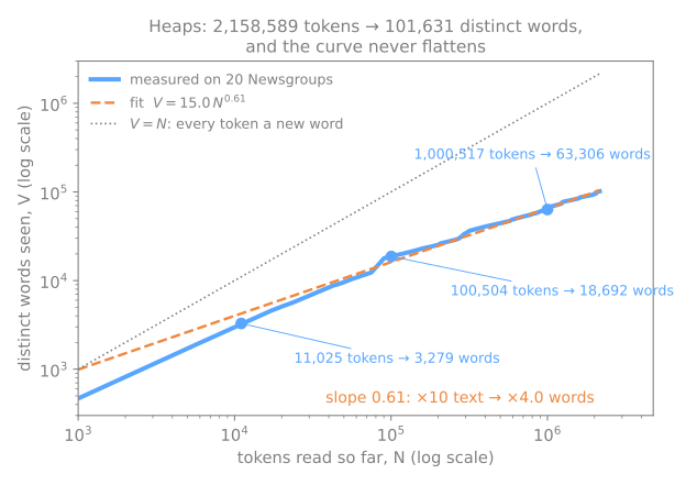
how to read it
- x axis: tokens read so far; y axis: distinct words seen. Both on a log scale.
- On a log scale a power law is a straight line; its slope, 0.61, is the exponent.
- Dotted: if every token were a new word. The curve stays below it, but never lies down.
- 11 thousand tokens → 3,279 words; 100 thousand → 18,692; 1 million → 63,306.
Zipf's law: a few words are everywhere
Predict. Of the 101,631 distinct words, what share occurs exactly once in the whole corpus: 5%, 25%, or more than half?
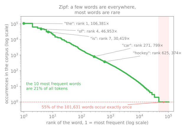
how to read it
- Each point is a word. x axis: its rank (1 = most frequent); y axis: how many times it occurs. Both on a log scale.
- At the top, "the" (106,381 times), "of", "is": the first 10 are 21% of all tokens.
- In the middle, "car" (rank 271, 799 times) and "hockey" (rank 625, 374 times).
- Red band: 55% of the words occur exactly once.
Simulator: tokenize a paragraph
Predict. Switch from unigrams to uni + bi, what ngram_range=(1, 2) does: does the vocabulary grow a little, double, or more?
A map of the approaches
Once the text is cut into tokens, four pages turn the tokens into vectors, from the simplest to the most powerful. Point at a family to follow it.
What each one does, and cannot do
| page | a document becomes | built from | what it cannot do |
|---|---|---|---|
| U4.1 Bag-of-words | its word counts, one column per word | counting, no model | see word order, synonyms, or words not seen in fit |
| U4.2 TF-IDF | counts weighted by how rare each word is | counting over the corpus | the same: it only reweights the columns |
| U4.3 Word embeddings | a dense vector per word (averaged for a document) | co-occurrence in a large corpus | tell apart the senses of one word |
| U4.4 Sentence embeddings | one dense vector per sentence or short document | a pretrained transformer | be cheap, or explain its dimensions |
Bag-of-words: a document is its counts
       cachorro  comeu  do  dorme  gato  peixe  ração  sonha
doc 1         0      1   0      0     1      1      0      0
doc 2         1      1   1      0     1      0      1      0
doc 3         0      0   0      1     2      0      0      1
- One row per document, one column per word; "gato" is 2 in document 3. Word order is thrown away.
- 13 of the 24 cells are already zero. The 11,314 posts: \(11{,}314 \times 101{,}631\), 99.90% zeros, stored in a sparse format.
TF-IDF: counts weighted by rarity
\[ \text{tf-idf}(t, d) = \text{tf}(t, d) \times \Big(\ln \frac{1 + n}{1 + \text{df}(t)} + 1\Big) \]then each row is divided by its length. Predict. In document 1 (gato, comeu, peixe: one each), which word weighs most?
     cachorro   comeu      do   dorme  gato   peixe   ração   sonha
idf    1.6931  1.2877  1.6931  1.6931   1.0  1.6931  1.6931  1.6931
       cachorro  comeu     do  dorme   gato  peixe  ração  sonha
doc 1     0.000  0.548  0.000  0.000  0.425   0.72  0.000  0.000
doc 2     0.505  0.384  0.505  0.000  0.298   0.00  0.505  0.000
doc 3     0.000  0.000  0.000  0.543  0.641   0.00  0.000  0.543
"peixe", only in document 1, weighs 0.720; "gato", in all three, 0.425. Same zeros, each row of length 1. Spärck Jones (1972); Salton & Buckley (1988).
Similarity and distance: four measures
cosine similarity
compares the directions of the two vectors, ignores their lengths. 1 = same words in the same proportions; 0 = nothing in common.
Euclidean distance
the straight-line distance between the two points (the one k-means uses). 0 = identical; grows with every difference, including length.
dot product
multiply coordinate by coordinate and add. Large when both are large in the same columns: grows with document length.
Jaccard similarity
forget counts, compare the sets of tokens: shared tokens over all distinct tokens.
A query and two candidates
Columns: cachorro, comeu, do, dorme, gato, peixe, ração, sonha. The query is A.
| A = "O gato comeu o peixe." | [0 1 0 0 1 1 0 0] |
| B = "Gato dorme, gato sonha." (another subject) | [0 0 0 1 2 0 0 1] |
| A3 = A written three times (same subject, longer) | [0 3 0 0 3 3 0 0] |
| pair | cosine | Euclidean | dot | Jaccard |
|---|---|---|---|---|
| A and B | 0.471 | 2.236 | 2 | 0.200 |
| A and A3 | 1.000 | 3.464 | 9 | 1.000 |
| B and A3 | 0.471 | 4.583 | 6 | 0.200 |
Why the cosine is the default for text
- Cosine: A3 is identical to A (1.000), B a partial match (0.471); B scores 0.471 against A and A3 alike.
- Euclidean gets it backwards: A3 is farther from A (3.464) than B (2.236), only because it is longer.
- Dot product: B against A3 scores 6, three times its 2 against A, for the same content.
- Jaccard agrees here, but it is blind to how often a word appears.
normalize_embeddings=True.The limits of sparse representations
- Synonyms score zero: cosine 0.00. Every word is its own axis, orthogonal to the others.
- Word order is invisible: "the dog bit the man" and "the man bit the dog" have cosine 1.00.
- One spelling, two meanings: manga (sleeve or mango) makes unrelated sentences look alike, and two sentences with the same meaning look unrelated (0.14 in both cases).
- New words vanish: a word not seen in
fithas no column.
Dense: know a word by its company
"You shall know a word by the company it keeps" (Firth, 1957)
- Distributional hypothesis (Harris, 1954): words used in similar contexts have similar meanings.
- "car" and "automobile" rarely share a sentence, but both appear next to engine, dealer, tires.
- Each word or text gets a few hundred numbers, learned so that similar contexts give nearby vectors.
Word embeddings, sentence embeddings
word embeddings (U4.3)
word2vec (Mikolov et al., 2013) predicts the words around each word; GloVe factorizes co-occurrence counts.
Synonyms end up close. Limit: one vector per word, whatever its sense.
sentence embeddings (U4.4)
Transformers (BERT) compute each token from the whole sentence: manga next to "camisa" ≠ next to "madura".
Sentence-BERT: one vector per sentence; the cosine tracks closeness of meaning.
Word embeddings: what a vector looks like
GloVe, trained on 6 billion tokens of English text: 400,000 words, 50 numbers each.
glove = api.load('glove-wiki-gigaword-50')
print('cat =', glove['cat'][:8].round(3), '...')
print(glove.most_similar('cat', topn=5))
cat = [ 0.453 -0.501 -0.537 -0.016  0.222  0.546 -0.673 -0.689] ... (50 numbers, none of them zero)
nearest to cat: dog 0.92, rabbit 0.85, monkey 0.80, rat 0.79, cats 0.79
cosine car / automobile: 0.70
cosine car / banana: 0.22
No single number means anything; the neighbors do. "car" and "automobile" never shared a bag-of-words column; here they have cosine 0.70.
Sentence embeddings: one vector per sentence
paraphrase-multilingual-MiniLM-L12-v2, with normalize_embeddings=True: 384 numbers per text, 50+ languages.
(3, 384)
o carro é rápido = [ 0.016  0.033 -0.08   0.037 -0.014 -0.002  0.039 -0.028] ... (384 numbers)
vs 1: cosine 0.97 · dot 0.97 · Euclidean 0.25
vs 2: cosine 0.23 · dot 0.23 · Euclidean 1.24
At length 1, dot product = cosine, and the Euclidean distance tells the same story in reverse.
Sparse vs dense: one sentence, three vectors
"the cat sleeps on the couch": bag-of-words over the newsgroups' vocabulary, the average of its GloVe vectors, its sentence embedding.
| length | non-zero | values | |
|---|---|---|---|
| bag-of-words | 101,631 | 5 | cat (column 26,019) = 1, couch = 1, on = 1, sleeps = 1, the = 2 · all others 0 |
| GloVe average | 50 | 50 | [ 0.271 0.037 -0.335 -0.147 0.541 0.055] ... |
| sentence embedding | 384 | 384 | [ 0.39 -0.348 -0.135 0.145 0.115 0.278] ... |
What "sparse" and "dense" mean
| sparse (bag-of-words, TF-IDF) | dense (word and sentence embeddings) | |
|---|---|---|
| length | one column per vocabulary word: 101,631 | fixed by the model: 50 (GloVe), 384 (sentence) |
| non-zero values | only the words of the text: 5 | all of them |
| one coordinate means | column 26,019 = "how many times cat appears" | nothing on its own |
| stored as | the non-zero cells (index, value) | a plain array of floats |
| no word in common | no shared column: cosine 0 | can still be close |
Simulator: four ways to turn a sentence into a vector
Predict. On the paraphrase "the car is fast" / "this automobile goes quickly", which of the four gives cosine 0? Then swap the word order and tick B three times.
Sparse vs dense: the same pairs, both ways
TF-IDF fitted on the sentences of the table; a small multilingual sentence-transformers model (384 numbers per text).
| A | B | TF-IDF | embedding |
|---|---|---|---|
| o carro é rápido | o automóvel é veloz | 0.00 | 0.97 |
| comprei um celular novo | adquiri um smartphone novo | 0.43 | 0.91 |
| o gato dorme no sofá | the cat sleeps on the couch | 0.00 | 0.98 |
| a manga da camisa rasgou | o punho da blusa descosturou | 0.21 | 0.87 |
| a manga da camisa rasgou | comi uma manga madura | 0.21 | 0.35 |
| o filme é muito bom | o filme não é bom | 0.60 | 0.46 |
| o cachorro mordeu o homem | o homem mordeu o cachorro | 1.00 | 0.98 |
| a taxa de juros subiu | o time venceu o jogo | 0.00 | 0.14 |
Reading the table, row by row
- paraphrases: 0.91 against 0.43; TF-IDF only sees "um" and "novo".
- translation: no token in common, 0.98. A Portuguese query can find English documents.
- the two "manga" rows: TF-IDF gives both 0.21; the embedding separates sleeve-and-cuff (0.87) from sleeve-and-mango (0.35).
- negation: lower (0.46), but far from "opposite".
- word order: 0.98. Embeddings blur who bit whom too.
- unrelated: 0.14, not 0.
Where TF-IDF is stronger: exact rare tokens
Two help-desk entries that differ only in an error code (0x80070005 vs 0x80004005), and a query for each code.
TF-IDF
embedding
Classification: how many labels do you have?
Four newsgroups, a logistic regression used as a black box; only the representation changes. Accuracy on 1,364 later posts (guessing one class: about 25%).
| labeled posts per class | TF-IDF + clf | embedding + clf |
|---|---|---|
| 5 | 0.557 | 0.819 |
| 10 | 0.601 | 0.851 |
| 25 | 0.725 | 0.886 |
| 100 | 0.850 | 0.897 |
| all | 0.904 | 0.901 |
Why: what each one arrives knowing
TF-IDF, 20 training posts
has seen only a few hundred distinct words; a test post that uses none of them is a zero vector. With all the labels, it learns each class's vocabulary from the data.
embedding
arrives already knowing that "sedan" is near "car", from the text it was trained on.
Sparse vs dense, side by side
| sparse (bag-of-words, TF-IDF) | dense (sentence embeddings) | |
|---|---|---|
| a document vector | \(\lvert V \rvert\) columns, 99.9% zeros | 384–1,024 numbers |
| synonyms, paraphrases | orthogonal: 0.00 | nearby: 0.97 |
words never seen in fit | dropped | handled (subword pieces) |
| rare exact tokens | high idf, strong signal | blurred into the meaning |
| other languages | separate vocabularies | shared space (multilingual model) |
| 5 labels per class / all | 55.7% / 90.4% | 81.9% / 90.1% |
| interpretability | each column is a word | columns are abstract |
| cost | fractions of a second, no model | a pretrained model; a GPU helps |
Summary: which one, when
- Start with TF-IDF: cheap and hard to beat when labels and domain vocabulary are plentiful.
- Reach for embeddings when meaning matters more than exact words (search, short texts, paraphrases, several languages) or labels are scarce.
- When exact tokens and meaning matter, combine them.
Sparse vs dense on real posts
- Four newsgroups (computer graphics, baseball, electronics, Christianity), about 2,100 posts, represented twice: TF-IDF and sentence embeddings.
- Steps: load the posts · two representations · which one finds posts about the same subject? · semantic vs keyword search · look at the two spaces · the same black-box classifier on both.
- Download the lab notebook and open it in Jupyter or Colab; in Colab, run
!pip install sentence-transformersfirst.
Each of the four sub-pages (U4.1 to U4.4) has its own simulator and lab.