U4.2 TF-IDF

The bag-of-words ended with two problems in one figure: raw counts are led by words that are in every document ("the", in 9,475 of 11,314 posts), and a single strange document can dominate a column ("ax", 62,387 occurrences in 20 posts). A stop list fixes the first problem for one language, and only for the words someone thought of listing. TF-IDF (term frequency × inverse document frequency) fixes both with one rule learned from the corpus itself: a word weighs more in a document the more often it occurs there, and less the more documents contain it.

This page computes TF-IDF by hand on three sentences, checks that scikit-learn gives exactly the same numbers, compares documents with the cosine, builds a small search engine, and measures where the whole sparse approach breaks down. Every number comes from running the code next to it.

The lesson follows one pipeline in four stages, drawn below: 1. weigh the words, the idea and the idf formula; 2. compute and check, every number by hand and then in scikit-learn; 3. compare and search, with the cosine and a small search engine; 4. where it breaks, the failures of every sparse representation. Each stage links to its section, and in the slides a strip at the bottom shows which stage you are in.

Weigh the wordstf × idf, the idf curve
Compute and checkthree sentences by hand, scikit-learn, three knobs
Compare and searchcosine, a small search engine, a real corpus
Where it breakssynonyms, word order, two meanings, unseen words

Slides

Click the slides and use the ← → arrows to navigate; F goes full screen and Esc shows every slide. Open the slides in a new tab

The idea: weigh words by how specific they are

Stage 1. The idea is Spärck Jones's (1972): a term that occurs in many documents is a poor way to tell documents apart, so it should count less. She measured it in retrieval experiments, and Salton & Buckley (1988), comparing many weighting schemes on several collections, made tf × idf with length normalization the standard of information retrieval.

scikit-learn's default version, for a word \(t\) in a document \(d\), in a corpus of \(n\) documents of which \(\text{df}(t)\) contain \(t\):

\[ \text{tf-idf}(t, d) = \underbrace{\text{tf}(t, d)}_{\text{count of } t \text{ in } d} \times \underbrace{\Big(\ln \frac{1 + n}{1 + \text{df}(t)} + 1\Big)}_{\text{idf}(t)} \]

and then every document vector is divided by its Euclidean length, so that each row has norm 1 (norm='l2'). Two details differ from the textbook \(\ln(n/\text{df})\):

the "+1" inside the fraction (smooth_idf=True) acts as if one extra document contained every word once: no division by zero, and a slightly flatter curve;
the "+1" outside keeps a word present in every document at weight 1 instead of 0. It is discounted, not deleted.

(figure script)

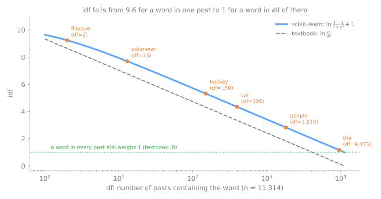
The curve is logarithmic: going from 1 post to 10 costs about as much weight as going from 1,000 to 10,000. A word that appears in 2 posts ("filioque", a term of Christian theology) gets an idf of 9.2, almost 8 times the 1.18 of a word that appears in nearly all of them ("the").

By hand, on three sentences

Stage 2. The three documents of the bag-of-words page and their counts:

import numpy as np
import pandas as pd
from sklearn.feature_extraction.text import CountVectorizer

docs = ["O gato comeu o peixe.",                 # the cat ate the fish
        "O cachorro comeu a ração do gato.",     # the dog ate the cat's food
        "Gato dorme, gato sonha."]               # cat sleeps, cat dreams
bow = CountVectorizer()
X = bow.fit_transform(docs)
print(pd.DataFrame(X.toarray(), columns=bow.get_feature_names_out(), index=['d1', 'd2', 'd3']))

    cachorro  comeu  do  dorme  gato  peixe  ração  sonha
d1         0      1   0      0     1      1      0      0
d2         1      1   1      0     1      0      1      0
d3         0      0   0      1     2      0      0      1

With \(n = 3\), there are only three possible values of idf:

"gato", in all 3 documents: \(\ln(4/4) + 1 = 1\);
"comeu", in 2 documents: \(\ln(4/3) + 1 = 1.2877\);
every other word, in 1 document: \(\ln(4/2) + 1 = 1.6931\).

For d1 ("gato comeu peixe", each word once), tf × idf gives gato 1, comeu 1.2877, peixe 1.6931. Its length is \(\sqrt{1^2 + 1.2877^2 + 1.6931^2} = \sqrt{5.5249} = 2.3505\), and dividing by it gives 0.4254, 0.5478, 0.7203. The rarest word of d1 now has the largest weight. The same steps in NumPy:

n = len(docs)
df = (X.toarray() > 0).sum(axis=0)              # in how many documents each word appears
idf = np.log((1 + n) / (1 + df)) + 1            # scikit-learn's smoothed idf, natural log
for word, d, i in zip(bow.get_feature_names_out(), df, idf):
    print(f"{word:9s} df = {d}   idf = {i:.4f}")

cachorro  df = 1   idf = 1.6931
comeu     df = 2   idf = 1.2877
do        df = 1   idf = 1.6931
dorme     df = 1   idf = 1.6931
gato      df = 3   idf = 1.0000
peixe     df = 1   idf = 1.6931
ração     df = 1   idf = 1.6931
sonha     df = 1   idf = 1.6931

w = X.toarray()[0] * idf                        # d1: raw count x idf
print('tf x idf :', w.round(4))
print(f'length   : {np.linalg.norm(w):.4f}')
print('tf-idf   :', (w / np.linalg.norm(w)).round(4))

tf x idf : [0.     1.2877 0.     0.     1.     1.6931 0.     0.    ]
length   : 2.3505
tf-idf   : [0.     0.5478 0.     0.     0.4254 0.7203 0.     0.    ]

scikit-learn confirms

TfidfVectorizer is CountVectorizer followed by exactly this weighting:

from sklearn.feature_extraction.text import TfidfVectorizer

tfidf = TfidfVectorizer()          # defaults: smooth_idf=True, norm='l2', sublinear_tf=False
T = tfidf.fit_transform(docs)
print(pd.DataFrame(T.toarray(), columns=tfidf.get_feature_names_out(), index=['d1', 'd2', 'd3']).round(4))
print('same idf as by hand:', np.allclose(tfidf.idf_, idf))

    cachorro   comeu      do   dorme    gato   peixe   ração   sonha
d1    0.0000  0.5478  0.0000  0.0000  0.4254  0.7203  0.0000  0.0000
d2    0.5046  0.3838  0.5046  0.0000  0.2980  0.0000  0.5046  0.0000
d3    0.0000  0.0000  0.0000  0.5427  0.6411  0.0000  0.0000  0.5427
same idf as by hand: True

Row d1 matches the hand computation to the fourth decimal, and idf_ holds the idf of every column.

(figure script)

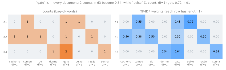
Two things to read in the figure. In d1 and d2, "gato" now has the smallest non-zero weight, because it is everywhere. In d3 it still has the largest (0.64): it occurs twice, and tf still counts. The weighting does not remove common words; it lowers them relative to rare ones.

Three knobs

for params in [{}, {'smooth_idf': False}, {'sublinear_tf': True}, {'norm': None}]:
    V = TfidfVectorizer(**params).fit_transform(docs)
    print(f"{str(params):24s} d3 = {V.toarray()[2].round(4)}")

{}                       d3 = [0.     0.     0.     0.5427 0.6411 0.     0.     0.5427]
{'smooth_idf': False}    d3 = [0.     0.     0.     0.5864 0.5588 0.     0.     0.5864]
{'sublinear_tf': True}   d3 = [0.     0.     0.     0.5774 0.5774 0.     0.     0.5774]
{'norm': None}           d3 = [0.     0.     0.     1.6931 2.     0.     0.     1.6931]

smooth_idf=False uses \(\ln(n/\text{df}) + 1\): the rare words of d3 get \(\ln 3 + 1 = 2.0986\) instead of 1.6931, while "gato" stays at 1. They overtake it: 0.5864 against 0.5588;
sublinear_tf=True replaces the count by \(1 + \ln(\text{tf})\): the two occurrences of "gato" count \(1 + \ln 2 = 1.6931\) instead of 2. By coincidence that equals the idf of the rare words, so the three weights of d3 become equal (0.5774 each). A word repeated many times can no longer take over its row;
norm=None keeps the raw products, and the rows no longer have length 1. Longer documents then have larger vectors, which matters for the Euclidean distance but not for the cosine.

Comparing documents: cosine similarity

Stage 3. The bag-of-words page introduced the cosine between two vectors, \(\cos(x_a, x_b) = x_a \cdot x_b / (\lVert x_a \rVert \lVert x_b \rVert)\). TF-IDF rows already have length 1, so the cosine is just their dot product. By hand, d1 and d2 share comeu and gato:

\[ \cos(d_1, d_2) = 0.5478 \times 0.3838 + 0.4254 \times 0.2980 = 0.2102 + 0.1268 = 0.337 \]

and d1 and d3 share only gato: \(0.4254 \times 0.6411 = 0.273\). Side by side with the cosines of the raw counts:

from sklearn.metrics.pairwise import cosine_similarity

names = ['d1', 'd2', 'd3']
print('counts\n', pd.DataFrame(cosine_similarity(X), index=names, columns=names).round(3))
print('TF-IDF\n', pd.DataFrame(cosine_similarity(T), index=names, columns=names).round(3))

counts
        d1     d2     d3
d1  1.000  0.516  0.471
d2  0.516  1.000  0.365
d3  0.471  0.365  1.000
TF-IDF
        d1     d2     d3
d1  1.000  0.337  0.273
d2  0.337  1.000  0.191
d3  0.273  0.191  1.000

Every similarity went down, because every shared word here includes "gato", which TF-IDF discounts. The pair d1–d3 dropped the most (0.471 → 0.273): what they share is only "gato", the least informative word of the corpus, and "gato" appears twice in d3.

A small search engine

Retrieval is what TF-IDF was invented for: turn the query into a vector with the same fitted vectorizer, and rank the documents by cosine. A help-desk FAQ of ten questions, and five queries written the way a student would type them:

faq = ["Como faço para trocar a senha do portal do aluno?",
       "Qual é o prazo para trancar a matrícula?",
       "Onde consigo a segunda via do boleto da mensalidade?",
       "Como peço revisão da nota de uma prova?",
       "O restaurante do campus abre aos sábados?",
       "Como reservo uma sala de estudos na biblioteca?",
       "Posso levar um visitante ao campus?",
       "Como justifico uma falta por motivo de saúde?",
       "O que fazer quando aparece o erro 0x80070005 na instalação?",
       "O que fazer quando aparece o erro 0x80004005 na atualização?"]
queries = ["esqueci minha senha",                    # I forgot my password
           "erro 0x80004005",                        # error 0x80004005
           "quero contestar a correção do exame",    # I want to contest the grading of the exam
           "onde almoçar no sábado",                 # where to have lunch on Saturday
           "perdi a fatura"]                         # I lost the invoice

tf_faq = TfidfVectorizer().fit(faq)
F = tf_faq.transform(faq)
for q in queries:
    sims = cosine_similarity(tf_faq.transform([q]), F).ravel()
    best = sims.argmax()
    used = [w for w in tf_faq.build_analyzer()(q) if w in tf_faq.vocabulary_]
    print(f"{q:37s} {sims[best]:.2f}  FAQ {best}: {faq[best][:45]:45s} words used: {used}")

esqueci minha senha                   0.35  FAQ 0: Como faço para trocar a senha do portal do al words used: ['senha']
erro 0x80004005                       0.53  FAQ 9: O que fazer quando aparece o erro 0x80004005  words used: ['erro', '0x80004005']
quero contestar a correção do exame   0.51  FAQ 0: Como faço para trocar a senha do portal do al words used: ['do']
onde almoçar no sábado                0.37  FAQ 2: Onde consigo a segunda via do boleto da mensa words used: ['onde']
perdi a fatura                        0.00  FAQ 0: Como faço para trocar a senha do portal do al words used: []

Two queries work, three fail, and the last column says why:

"esqueci minha senha" finds the password question through "senha", and the error code finds its own entry: a rare token has a high idf, so an exact code is the ideal TF-IDF query;
"quero contestar a correção do exame" shares only "do" with the FAQ, and the password question, which contains "do" twice, wins with 0.51. The right answer ("revisão da nota de uma prova") uses none of the query's words;
"onde almoçar no sábado" matches the invoice question through "onde" (where), because the restaurant entry says "sábados", not "sábado". A stemmer would fix this one;
"perdi a fatura" has no word in common with any entry: similarity 0.00 with everything, and argmax returns the first question by default.

A stop list removes the false matches but cannot create true ones:

stop_pt = ['o', 'a', 'os', 'as', 'do', 'da', 'de', 'no', 'na', 'e', 'um', 'uma', 'em', 'que',
           'como', 'para', 'onde', 'qual', 'quero', 'minha']
tf_stop = TfidfVectorizer(stop_words=stop_pt).fit(faq)
for q in queries[2:4]:
    sims = cosine_similarity(tf_stop.transform([q]), tf_stop.transform(faq)).ravel()
    print(f"{q:37s} best score {sims.max():.2f}")

quero contestar a correção do exame   best score 0.00
onde almoçar no sábado                best score 0.00

With the function words gone, the two queries score 0.00 with every entry: TF-IDF now honestly says it found nothing. Keyword search can only be as good as the overlap between the words of the query and the words of the documents.

On a real corpus

The same comparison at scale: 2,097 posts from four newsgroups (cars, medicine, space, guns), represented by raw counts or by TF-IDF, reduced to 50 dimensions with a truncated SVD and drawn with t-SNE. The newsgroup is used only for the color:

(figure script)

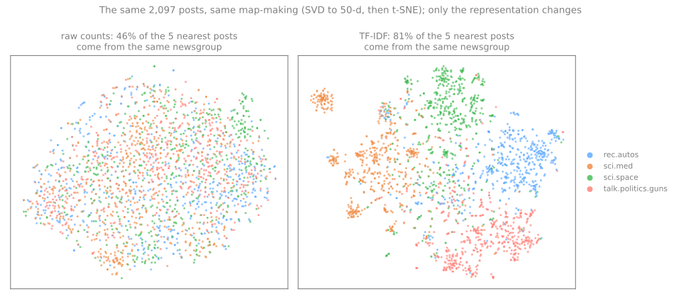
With raw counts, the nearest posts are those that use the, of, and in similar proportions: only 46% of each post's 5 nearest neighbors come from its newsgroup (a random pick would give about 25%). TF-IDF, which discounts exactly those words, raises it to 81%, and four regions appear on the map.

The limits of sparse representations

Stage 4. TF-IDF is fast, needs no training data, and is easy to read: every column is a word you can print. Its weakness comes from the construction itself: each word is its own axis, orthogonal to every other word. Four measured consequences, each on a pair of sentences:

analyzer = CountVectorizer().build_analyzer()
pairs = {'synonyms':     ("o carro é rápido", "o automóvel é veloz"),
         'word order':   ("o cachorro mordeu o homem", "o homem mordeu o cachorro"),
         'two meanings': ("a manga da camisa rasgou", "comi uma manga madura"),
         'same meaning': ("a manga da camisa rasgou", "o punho da blusa descosturou")}
for name, (a, b) in pairs.items():
    V = TfidfVectorizer().fit_transform([a, b])
    shared = sorted(set(analyzer(a)) & set(analyzer(b)))
    print(f"{name:13s} cosine {cosine_similarity(V)[0, 1]:.2f}   shared words: {shared}")

synonyms      cosine 0.00   shared words: []
word order    cosine 1.00   shared words: ['cachorro', 'homem', 'mordeu']
two meanings  cosine 0.14   shared words: ['manga']
same meaning  cosine 0.14   shared words: ['da']

Synonyms score zero. "The car is fast" and "the automobile is quick" share no token ("é" has one letter), so their similarity is exactly 0.00.
Order is invisible. Who bit whom does not change the vector: 1.00.
One spelling, two meanings. Manga is a sleeve in "the shirt's sleeve tore" and a mango in "I ate a ripe mango". The two sentences share that token and score 0.14.
Same meaning, different words. "The sleeve of the shirt tore" and "the cuff of the blouse came unstitched" describe almost the same event, share only the preposition "da", and also score 0.14. TF-IDF cannot tell the related pair from the unrelated one.

And a fifth: words never seen during fit have no column. With the vectorizer fitted on the three documents of this page:

for new in ["o cachorro latiu", "um felino adormeceu"]:          # "the dog barked", "a feline fell asleep"
    v = tfidf.transform([new])
    print(f"{new!r:24s} non-zeros: {v.nnz}   {dict(zip(tfidf.get_feature_names_out()[v.indices], v.data.round(2).tolist()))}")

'o cachorro latiu'       non-zeros: 1   {'cachorro': 1.0}
'um felino adormeceu'    non-zeros: 0   {}

"latiu" is dropped, and "a feline fell asleep" becomes the zero vector: a sentence about a cat sleeping, next to documents about cats sleeping, with similarity 0 to all of them. By Heaps' law, new words never stop arriving.

These are the failures that motivated dense representations, where words and sentences with similar meaning get nearby vectors even when they share no token: word embeddings and sentence embeddings. The overview measures when each family wins.

Simulator: TF-IDF and search, live

Type one document per line, and a query below. The simulator computes df, idf, the TF-IDF matrix, the cosine between documents and the ranking of the query exactly as TfidfVectorizer does, with the three knobs of this page.

Things to try:

the lesson preset reproduces the numbers above (idf 1, 1.288, 1.693; d1 = 0.548, 0.425, 0.720; cos(d1, d2) = 0.337). Untick smooth_idf and watch the idf of the rare words go up;
add a fourth line that repeats "gato" five times, and tick sublinear_tf: how much does the repetition still count?
the synonyms preset: "carro veloz" matches the second sentence only through "veloz", and the first only through "carro"; neither is recognized as meaning the same thing;
the FAQ preset: the query finds the invoice question through "onde", and "sábado" is ignored because the documents only contain "sábados".

Exercises

By hand, compute the TF-IDF row of d3 ("Gato dorme, gato sonha.") and check 0.6411, 0.5427, 0.5427. Then compute \(\cos(d_2, d_3)\) and check 0.191.
Add a fourth document, "O peixe dorme.", to the three of this page. Which idf values change? Why does the weight of "gato" in d1 go up, although d1 did not change?
With sublinear_tf=True, what is the weight of a word that occurs 10 times, relative to one that occurs once (same idf)? Compare with the raw count.
In the search engine above, add "almoço" to the restaurant entry. Does "onde almoçar no sábado" now find it? Explain with the tokens.

Lab: a TF-IDF search engine on real posts

Four newsgroups of the 20 Newsgroups collection (computer graphics, baseball, electronics and Christianity), about 2,100 posts. The lab builds the TF-IDF matrix, reads what it considers important, finds the most similar posts, measures how each option changes the quality of the neighbors, and turns the matrix into a keyword search engine, including a query it cannot answer. It uses only scikit-learn and runs in well under a minute.

Run the blocks in order, in one session. To work on it directly, download the lab notebook and open it in Jupyter or Colab (File → Upload notebook).

Step 1 — load the posts

import numpy as np
import pandas as pd
from sklearn.datasets import fetch_20newsgroups

cats = ['comp.graphics', 'rec.sport.baseball', 'sci.electronics', 'soc.religion.christian']
raw = fetch_20newsgroups(subset='train', categories=cats,
                         remove=('headers', 'footers', 'quotes'), random_state=0)
keep = [i for i, t in enumerate(raw.data) if len(t.split()) >= 20]   # drop empty/very short posts
docs = [raw.data[i] for i in keep]
y = raw.target[keep]
names = np.array(raw.target_names)
print(len(docs), 'posts:', ', '.join(f"{g} {c}" for g, c in zip(names, np.bincount(y))))

2116 posts: comp.graphics 521, rec.sport.baseball 495, sci.electronics 535, soc.religion.christian 565

The same 2,116 posts as in the bag-of-words lab: four balanced groups, 495 to 565 posts each, with headers, signatures and quoted replies removed and posts shorter than 20 words dropped.

Step 2 — the TF-IDF matrix and its idf

from sklearn.feature_extraction.text import TfidfVectorizer

tfidf = TfidfVectorizer(stop_words='english', min_df=2)
T = tfidf.fit_transform(docs)
terms = tfidf.get_feature_names_out()
print(T.shape, f"{1 - T.nnz / (T.shape[0] * T.shape[1]):.2%} zeros")

idf = pd.Series(tfidf.idf_, index=terms).sort_values()
print('lowest idf :', idf.head(6).round(2).to_dict())
print(f"highest idf: {idf.iloc[-1]:.2f}, shared by the {(idf == idf.iloc[-1]).sum()} words found in exactly 2 posts")
print('row lengths:', np.sqrt(T.multiply(T).sum(axis=1)).A.ravel()[:5].round(3))

(2116, 12001) 99.52% zeros
lowest idf : {'like': 2.37, 'know': 2.41, 'don': 2.46, 'just': 2.49, 'think': 2.58, 'does': 2.62}
highest idf: 7.56, shared by the 3653 words found in exactly 2 posts
row lengths: [1. 1. 1. 1. 1.]

How to read it:

2,116 posts × 12,001 terms, 99.52% zeros. The English stop list and min_df=2 already halved the vocabulary; TF-IDF changes the values, not the sparsity.
The lowest idf values (2.37 to 2.62) belong to words that are not in the stop list but appear everywhere in informal writing: "like", "know", "just", "think". "don" is what the tokenizer leaves of "don't". TF-IDF discounts them automatically, without anyone listing them.
The highest idf is \(\ln(2117/3) + 1 = 7.56\), the value for a word found in exactly 2 posts, the minimum that min_df=2 allows. 3,653 words share it.
Every row has length 1: the L2 normalization, so a dot product between two rows is their cosine.

Step 3 — what a post is about, in eight words

i = 14
row = T[i].toarray().ravel()
print(f"post {i} ({names[y[i]]}):", ' '.join(docs[i].split())[:150])
print(pd.Series(row, index=terms).nlargest(8).round(3).to_string())

post 14 (sci.electronics): : >I want to upgrade my system and was thinking of buying Adcom seperates. : >I have heard from alot of people, though, that Adcom sounds great but :
adcom         0.463
amp           0.408
amplifier     0.270
components    0.250
amps          0.203
quality       0.165
sound         0.161
brilliant     0.151

Post 14 asks about buying Adcom audio amplifiers, and its eight heaviest terms read like a summary: the brand, "amp", "amplifier", "components", "sound". TF-IDF works as a keyword extractor: a word ranks high when this post uses it and few other posts do. "brilliant" (0.151) is a reminder that it knows nothing about meaning: an adjective the author happened to use, rare in the corpus, ranks next to the subject words.

Step 4 — the most similar posts

from sklearn.metrics.pairwise import cosine_similarity

sim = cosine_similarity(T[i], T).ravel()
sim[i] = -1                                         # skip the post itself
for j in np.argsort(-sim)[:3]:
    shared = [terms[k] for k in np.intersect1d(T[i].indices, T[j].indices)]
    print(f"{sim[j]:.2f}  {names[y[j]]:18s} shared terms: {shared[:8]}")

0.66  sci.electronics    shared terms: ['adcom', 'amp', 'amplifier', 'amplifiers', 'amps', 'brilliant', 'build', 'built']
0.37  sci.electronics    shared terms: ['amp', 'amps', 'components', 'designed', 'good', 'heat', 'hot', 'inside']
0.30  sci.electronics    shared terms: ['adcom', 'components', 'designed', 'east', 'far', 'like', 'people']

The three most similar posts all come from sci.electronics. The first (cosine 0.66) is a reply in the same discussion and shares the brand and the whole amplifier vocabulary; the second talks about amplifiers overheating ("heat", "hot"); the third about where Adcom builds its products ("far", "east"). The printed shared terms are the reason for each score: a cosine between TF-IDF rows is a sum over the words two posts have in common.

Step 5 — which options give the best neighbors?

from sklearn.feature_extraction.text import CountVectorizer
from sklearn.neighbors import NearestNeighbors

def agreement(V, k=5):
    """Share of each post's k nearest posts (cosine) that come from the same newsgroup."""
    nn = NearestNeighbors(n_neighbors=k + 1, metric='cosine').fit(V)
    _, idx = nn.kneighbors(V)
    return (y[idx[:, 1:]] == y[:, None]).mean()

print(f"chance level:                       {np.sum(np.bincount(y) ** 2) / len(y) ** 2:.3f}")
print(f"raw counts:                         {agreement(CountVectorizer().fit_transform(docs)):.3f}")
for params in [{'min_df': 2}, {'min_df': 2, 'max_df': 0.5}, {'stop_words': 'english', 'min_df': 2},
               {'stop_words': 'english', 'min_df': 2, 'sublinear_tf': True},
               {'stop_words': 'english', 'min_df': 2, 'ngram_range': (1, 2)}]:
    V = TfidfVectorizer(**params).fit_transform(docs)
    print(f"TF-IDF {str(params)[1:-1]:60s} {agreement(V):.3f}")

chance level:                       0.251
raw counts:                         0.490
TF-IDF 'min_df': 2                                                  0.770
TF-IDF 'min_df': 2, 'max_df': 0.5                                   0.829
TF-IDF 'stop_words': 'english', 'min_df': 2                         0.850
TF-IDF 'stop_words': 'english', 'min_df': 2, 'sublinear_tf': True   0.865
TF-IDF 'stop_words': 'english', 'min_df': 2, 'ngram_range': (1, 2)  0.843

The neighbor agreement of the bag-of-words lab: the share of each post's 5 nearest posts that come from its newsgroup (0.251 by chance).

Raw counts: 0.490. TF-IDF with no stop list: 0.770. The idf alone does most of the work of a stop list: the words in every post get weights near the bottom of the scale.
max_df=0.5: 0.829; the English stop list: 0.850. Removing the most common words outright still helps a little more.
sublinear_tf=True: 0.865, the best here: long posts that repeat a word many times no longer let it dominate.
Bigrams: 0.843, no better than words alone, as in the bag-of-words lab.

Step 6 — a keyword search engine

queries = {"my picture looks blurry after I enlarge it": 'comp.graphics',
           "software to convert a photo from one file format to another": 'comp.graphics',
           "the umpire made a terrible call last night": 'rec.sport.baseball',
           "why does my TV screen flicker": 'sci.electronics',
           "how to stop my circuit from overheating": 'sci.electronics',
           "does the soul survive after death": 'soc.religion.christian'}

def search(query, k=5):
    return np.argsort(-cosine_similarity(tfidf.transform([query]), T).ravel())[:k]

for q, group in queries.items():
    top = search(q)
    used = list(terms[tfidf.transform([q]).indices])
    print(f"{q}\n   {np.sum(names[y[top]] == group)}/5 from {group} · words used: {used}")

my picture looks blurry after I enlarge it
   3/5 from comp.graphics · words used: ['blurry', 'enlarge', 'looks', 'picture']
software to convert a photo from one file format to another
   5/5 from comp.graphics · words used: ['convert', 'file', 'format', 'photo', 'software']
the umpire made a terrible call last night
   3/5 from rec.sport.baseball · words used: ['night', 'terrible', 'umpire']
why does my TV screen flicker
   3/5 from sci.electronics · words used: ['does', 'screen', 'tv']
how to stop my circuit from overheating
   5/5 from sci.electronics · words used: ['circuit', 'stop']
does the soul survive after death
   2/5 from soc.religion.christian · words used: ['death', 'does', 'soul', 'survive']

Each query was written for one of the four groups, and we count how many of the 5 results come from that group: 21 out of 30. The last column explains the misses. Where the query uses the group's own vocabulary ("convert", "file", "format"; "circuit"), all 5 results are right. "flicker" and "overheating" are not in the vocabulary (fewer than 2 posts), so "why does my TV screen flicker" is searched as "does screen tv". And a Christian post rarely speaks of a "soul" that "survives" in those words, even when that is its subject: 2 out of 5.

Step 7 — what keyword search cannot see

col = tfidf.vocabulary_
for a, b in [('image', 'picture'), ('faith', 'belief')]:
    top_a, top_b = set(search(a, 10)), set(search(b, 10))
    n_a, n_b = (T[:, col[a]] > 0).sum(), (T[:, col[b]] > 0).sum()
    n_both = (T[:, col[a]] > 0).multiply(T[:, col[b]] > 0).sum()
    print(f"{a!r} in {n_a} posts, {b!r} in {n_b}, both in {n_both} · "
          f"top-10 results in common: {len(top_a & top_b)}")
print(tfidf.transform(["photograph of a luminous nebula"]).nnz, 'known words in the last query')

'image' in 90 posts, 'picture' in 39, both in 7 · top-10 results in common: 0
'faith' in 109 posts, 'belief' in 51, both in 22 · top-10 results in common: 0
0 known words in the last query

"image" and "picture" mean nearly the same thing in a graphics newsgroup, but only 7 posts contain both, and the 10 best results for one query share no post with the 10 best for the other. The same holds for "faith" and "belief". The last query, about a photograph of a nebula, has no word in the vocabulary of these four groups: its vector is zero, and every post scores 0. This is the limit of every sparse representation, and the reason for word embeddings and sentence embeddings.

Your turn

Your own queries. Write three queries for each newsgroup: one that reuses the group's vocabulary, one that paraphrases it, one with a typo. How many of the 5 results are right in each case?
Sublinear and stop words. Step 5 gave the best agreement with sublinear_tf=True. Check which words drop out of the top-8 of post 14 with that option, and explain why.
Query expansion. Make search add synonyms to the query before transforming it (for example, "picture" → "picture image photo"). Does step 7's top-10 overlap change? What is the risk of expanding every query?
Stemming. Install NLTK (pip install nltk), and pass tokenizer= a function that applies PorterStemmer().stem to each token. How many columns remain? Does the agreement of step 5 change?

Class materials

Lab notebook

The lab of this page as a notebook, ready for Jupyter or Colab: lab notebook.

References

Spärck Jones, K. "A Statistical Interpretation of Term Specificity and Its Application in Retrieval." Journal of Documentation 28, no. 1 (1972): 11–21 — the idea behind inverse document frequency. DOI
Salton, G.; Wong, A.; Yang, C. S. "A Vector Space Model for Automatic Indexing." Communications of the ACM 18, no. 11 (1975): 613–620 — documents as vectors, compared by cosine. DOI
Salton, G.; Buckley, C. "Term-Weighting Approaches in Automatic Text Retrieval." Information Processing & Management 24, no. 5 (1988): 513–523 — the systematic comparison that made tf × idf with length normalization the standard. DOI
Robertson, S. "Understanding Inverse Document Frequency: On Theoretical Arguments for IDF." Journal of Documentation 60, no. 5 (2004): 503–520 — why the logarithm, and what idf estimates. DOI
Manning, C. D.; Raghavan, P.; Schütze, H. Introduction to Information Retrieval. Cambridge University Press (2008) — chapter 6: term weighting and the vector space model. Full text
Lang, K. "NewsWeeder: Learning to Filter Netnews." Proceedings of ICML (1995): 331–339 — the origin of the 20 Newsgroups collection. DOI

U4.2 TF-IDF

Slides

The idea: weigh words by how specific they are

By hand, on three sentences

scikit-learn confirms

Three knobs

Comparing documents: cosine similarity

A small search engine

On a real corpus

The limits of sparse representations

Simulator: TF-IDF and search, live

Exercises

Lab: a TF-IDF search engine on real posts

Step 1 — load the posts

Step 2 — the TF-IDF matrix and its idf

Step 3 — what a post is about, in eight words

Step 4 — the most similar posts

Step 5 — which options give the best neighbors?

Step 6 — a keyword search engine

Step 7 — what keyword search cannot see

Your turn

Class materials

References

Quiz